DUC Wells and Their Economic Complications
Category > Oil and Gas
Feb 09, 2023Once a well is drilled, it must be completed to produce. However, operators may choose not to immediately complete a well for various reasons:
Availability of fracking crews
Drilling contracts that are too expensive to revoke
Constraints on capital spending
Commodity prices
Many others
Whatever the reasons may be, this in-transit time between drilling and completion stages creates an inventory of DUC wells. The term, DUC wells, have a literal definition - Drilled but Uncompleted wells. They essentially serve as a secodary form of hydrocarbon storage underground, instead of surface storage facilities. The wells can be turned on line for production for cheap; the costs of drilling have been paid, and completion won't be as costly as new drilling. This unique characteristic of DUC wells allows the operators to make strategic decisions during the time of financial crisis (ex: 2020 COVID crash); they complete the existing DUC wells and take profits instead of drilling new wells. However, this profit taking process inevitably leads to the reduction in size of DUC well inventories, which gave rise to the concerns regarding potential energy supply shortage due to the depletion of DUC wells around early 2022.
In this article I attempt to help the readers to understand what it means to have DUC well inventories, why they exist, and the economic impact they have on the US energy industry.
0. Sample data description
The main data source I use for this article is the Drilling Productivity Report (DPR) from the US Energy Information Administration (EIA), and some supplemental data from the Enverus Drilling Info application since 2014. While the DPR data is readily available to the public as its provided by the US government, Enverus' Drilling Info data is not because its a commerical software.
The DPR data covers the 7 major oil and gas basins in the US: Anadarko, Appalachia, Bakken, Eagle Ford, Haynesville, Niobrara, and Permian.
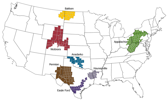
Figure 1: 7 major basins in the US, Source: EIA
I downloaded the Report data (aggregated by region) (dpr-data.xlsx) and the DUC data (aggregated by region) (duc-data.xlsx), which can be found in the "Contents" tab in the right side of this page. Visualizing the DPR data for each basin generates the below figure:
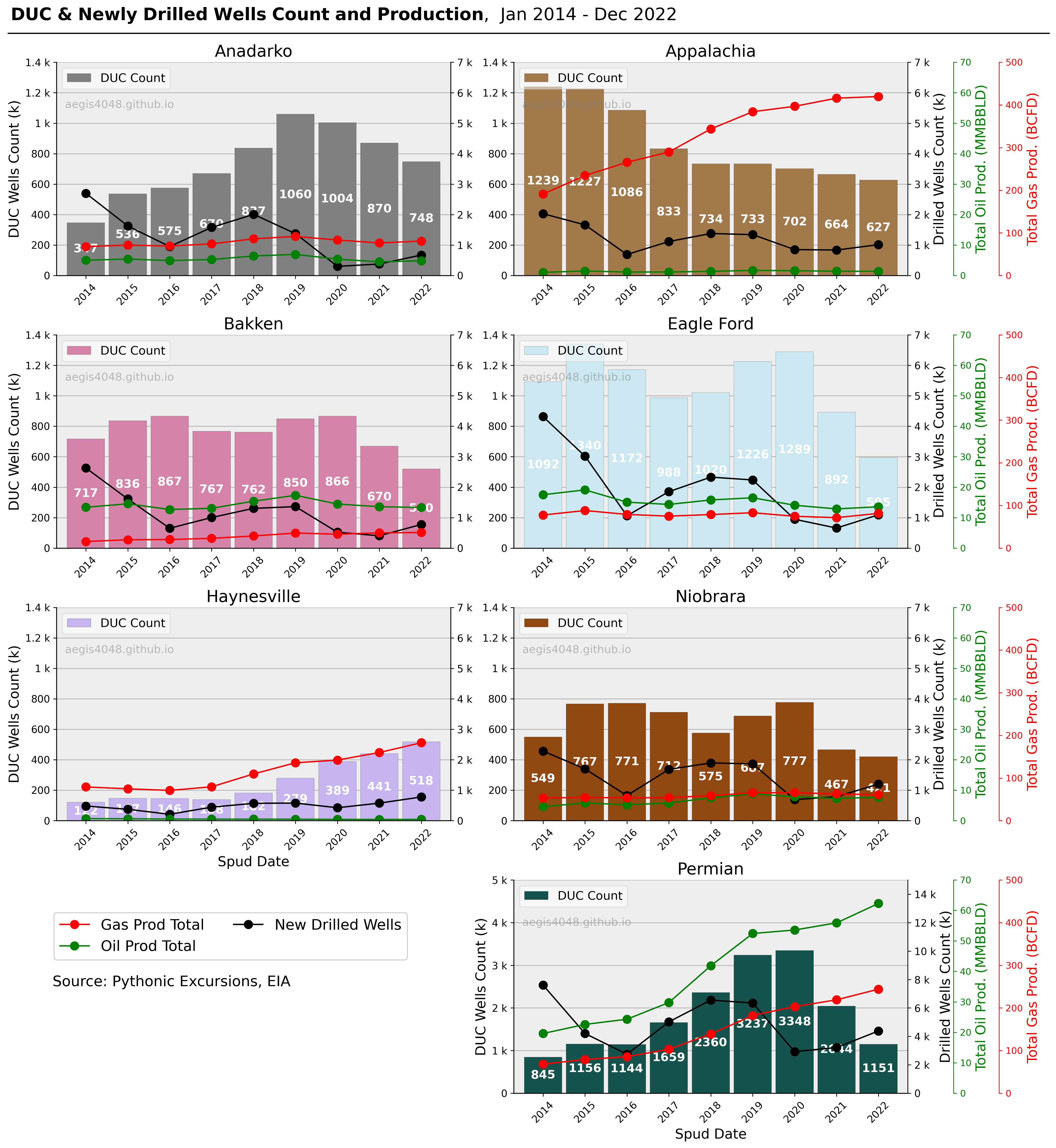
Figure 2: Quick glance at the EIA DPR data for each basin. Note that the Permian basin has different y-axis scale for DUC & newly drilled wells count.
Source Code For Figure (2)
import pandas as pd
import numpy as np
import matplotlib.pyplot as plt
import seaborn as sns
from matplotlib.colors import LinearSegmentedColormap
import warnings
import matplotlib.gridspec as gridspec
import matplotlib.ticker as ticker

############################################# Basins ##############################################

basins = sorted(['Anadarko', 'Appalachia', 'Eagle Ford', 'Haynesville', 'Niobrara', 'Permian', 'Bakken'])

################################### DUC Wells Count per Basin #####################################

# compile a DataFrame to store count of DUC wells per basin
# source: EIA - https://www.eia.gov/petroleum/drilling/

dfs = []
for basin in basins:
    df_cur = pd.read_excel('https://aegis4048.github.io/downloads/notebooks/sample_data/Duc-EIA.xlsx', sheet_name=basin)
    df_cur['Basin'] = basin
    dfs.append(df_cur)

df = pd.concat(dfs)
df = df.sort_values('Date')
df.index = pd.to_datetime(df['Date'])

df_DUCs_year = df.groupby([df.index.year, 'Basin'])['DUC'].mean()
df_DUCs_year = df_DUCs_year.unstack().fillna(0)
df_DUCs_year = round(df_DUCs_year, 0)

df_drilled_year = df.groupby([df.index.year, 'Basin'])['Drilled'].sum()
df_drilled_year = df_drilled_year.unstack().fillna(0)
df_drilled_year['Total Drilled'] = df_drilled_year.T.apply(lambda x: sum(x))

#################### Import All Data - Rig Count, Oil & Gas Prod per Basins #######################

dfs2 = []
for basin in basins:
    df_cur = pd.read_excel('https://aegis4048.github.io/downloads/notebooks/sample_data/dpr-data.xlsx', sheet_name=basin + ' Region', skiprows=1)
    df_cur['Basin'] = basin
    dfs2.append(df_cur)

year_cutoff = '2013' # counting from year_cutoff + 1
date_header = 'Month'

df2 = pd.concat(dfs2)
df2 = df2.sort_values(date_header)
df2.index = pd.to_datetime(df2[date_header])
df2.drop(df2.columns[[2, 3, 5, 6]], axis=1, inplace=True)
df2.columns = ['Date', 'Rig Count', 'Total Oil Prod (BBLD)', 'Total Gas Prod (MCFD)', 'Basin']
df2 = df2[df2.index > year_cutoff + '-12-31']

################################ Cross Table for Gas Production ###################################

# Total Gas Production
df2_total_gas_prod_year = df2.groupby([df2.index.year, 'Basin'])['Total Gas Prod (MCFD)'].sum()
df2_total_gas_prod_year = df2_total_gas_prod_year.unstack().fillna(0)
df2_total_gas_prod_year['Total Gas (BCFD)'] = df2_total_gas_prod_year.T.apply(lambda x: sum(x))
df2_total_gas_prod_year = df2_total_gas_prod_year / 1000000

################################ Cross Table for Oil Production ###################################

df2_total_oil_prod_year = df2.groupby([df2.index.year, 'Basin'])['Total Oil Prod (BBLD)'].sum()
df2_total_oil_prod_year = df2_total_oil_prod_year.unstack().fillna(0)
df2_total_oil_prod_year['Total (MMBBLD)'] = df2_total_oil_prod_year.T.apply(lambda x: sum(x))
df2_total_oil_prod_year = df2_total_oil_prod_year / 1000000

############################################# Plot ##############################################

# changing datetime index to str is necessary to overlay lineplot on top of barplot
df_drilled_year.index = [str(item) for item in df_drilled_year.index]
df2_total_gas_prod_year.index = [str(item) for item in df2_total_gas_prod_year.index]
df2_total_oil_prod_year.index = [str(item) for item in df2_total_oil_prod_year.index]

cmap_name = 'cubehelix'
colors = sns.color_palette(cmap_name, n_colors=len(basins))
np.random.seed(34)
np.random.shuffle(colors)
colors = colors.as_hex()
colors[0] = 'grey'
colors[-2] = '#914810'
cmap = LinearSegmentedColormap.from_list("my_colormap", colors)
barcolor_dict = {label: color for label, color in zip(basins, colors)}

axis_fontsize = 15
axis_tick_fontsize = 11
title_fontsize = 18
figure_title_fontsize = 20
label_fontsize = 13
legend_fontsize = 16
markersize = 9
y_label_fontsize = 15

gas_prod_color = 'red'
oil_prod_color = 'green'
drilled_color = 'k'

fig = plt.figure(figsize=(16, 17))
gs = gridspec.GridSpec(4, 4)
ax1 = plt.subplot(gs[0, 0:2])
ax2 = plt.subplot(gs[0,2:])
ax3 = plt.subplot(gs[1,0:2])
ax4 = plt.subplot(gs[1,2:])
ax5 = plt.subplot(gs[2,0:2])
ax6 = plt.subplot(gs[2,2:])
ax7 = plt.subplot(gs[3,2:4])
axes = [ax1,ax2,ax3,ax4,ax5,ax6,ax7]

for i, (ax, basin) in enumerate(zip(axes, basins)):

    df_DUCs_year.plot.bar(alpha=1, y=basin, ax=ax, legend=None, width=0.9, edgecolor='k', linewidth=0.1, label='DUC Count', color=barcolor_dict[basin])

    ax1 = ax.twinx()
    df_drilled_year.plot(y=basin, ax=ax1, linestyle='-', legend=None, marker='o', color=drilled_color, markersize=markersize, label='New Drilled Wells')

    ax2 = ax.twinx()
    df2_total_oil_prod_year.plot(y=basin, ax=ax2, linestyle='-', marker='o', color='green', markersize=markersize, label='Oil Prod Total', legend=None)
    ax2.set_ylim(0, 70)

    ax3 = ax.twinx()
    df2_total_gas_prod_year.plot(y=basin, ax=ax3, linestyle='-', marker='o', color='red', markersize=markersize, label='Gas Prod Total', legend=None)
    ax3.set_ylim(0, 500)

    ax.set_facecolor('#eeeeee')
    ax.set_axisbelow(True)
    ax.grid(axis='y')
    ax.set_xticklabels([str(dt).split('-')[0] for dt in df_DUCs_year.index])
    ax.tick_params(axis='x', labelrotation=45, labelsize=axis_tick_fontsize)
    ax.tick_params(axis='y', labelsize=axis_tick_fontsize)
    ax1.tick_params(axis='y', labelsize=axis_tick_fontsize)
    ax.set_title(basin, fontsize=title_fontsize)

    if i % 2 == 0 and i != 6:
        ax.set_ylabel('DUC Wells Count (k)', fontsize=axis_fontsize)
        ax2.set_yticks([])
        ax3.set_yticks([])
    else:
        ax1.set_ylabel('Drilled Wells Count (k)', fontsize=axis_fontsize)

        ax2.tick_params(axis='y', colors='green')
        ax2.spines['right'].set_position(('outward', 50))
        ax2.spines['right'].set_color('green')
        ax2.set_ylabel('Total Oil Prod. (MMBBLD)', color='green', fontsize= axis_fontsize)

        ax3.tick_params(axis='y', colors='red')
        ax3.spines['right'].set_position(('outward', 100))
        ax3.spines['right'].set_color('red')
        ax3.set_ylabel('Total Gas Prod. (BCFD)', color='red', fontsize= axis_fontsize)

    if i == 6:
        ax.set_ylabel('DUC Wells Count (k)', fontsize=axis_fontsize)
    #else:
        #ax1.set_yticks([])
        #ax2.set_yticks([])
        #ax3.set_yticks([])

    if i == 4 or i == 6:
        ax.set_xlabel('Spud Date', fontsize=y_label_fontsize)
    else:
        ax.set_xlabel('')

    if basin == 'Permian':
        pass
        ax.set_ylim(0, 5000)
        ax1.set_ylim(0, 15000)

    else:
        ax.set_ylim(0, 1400)
        ax1.set_ylim(0, 7000)

    ax.yaxis.set_major_formatter(ticker.EngFormatter())
    ax1.yaxis.set_major_formatter(ticker.EngFormatter())

    ax.spines.top.set_visible(False)
    ax1.spines.top.set_visible(False)
    ax2.spines.top.set_visible(False)
    ax3.spines.top.set_visible(False)

    #ax.yaxis.get_major_ticks()[-1].gridline.set_visible(False)
    #ax1.yaxis.get_major_ticks()[-1].gridline.set_visible(False)

    h0, l0 = ax.get_legend_handles_labels()
    h1, l1 = ax1.get_legend_handles_labels()
    h2, l2 = ax2.get_legend_handles_labels()
    h3, l3 = ax3.get_legend_handles_labels()
    ax.legend(h0, l0, loc='upper left', ncol=2, fontsize=13, framealpha=0.5)

    fig.legend(h3 + h2 + h1, l3 + l2 + l1, loc='lower left', ncol=2,
               bbox_to_anchor=(0.046, 0.165), bbox_transform=fig.transFigure, fontsize=legend_fontsize)

    for c in ax.containers:
        ax.bar_label(c, label_type='center', color='white', weight='bold', fontsize=label_fontsize)

    ax.text(0.16, 0.80, 'aegis4048.github.io', fontsize=12, ha='center', va='center',
            transform=ax.transAxes, color='grey', alpha=0.5)

fig.tight_layout()

def setbold(txt):
    return ' '.join([r"$\bf{" + item + "}$" for item in txt.split(' ')])

y_pos = 0.998
fig.suptitle(setbold('DUC & Newly Drilled Wells Count and Production')  + ",  Jan 2014 - June 2022", fontsize=19, x=0.328, y=1.025)
ax.annotate('', xy=(0.006, y_pos), xycoords='figure fraction', xytext=(1, y_pos), arrowprops=dict(arrowstyle="-", color='k', lw=1.3))
ax.annotate('Source: Pythonic Excursions, EIA', xy=(0.05, 0.145), xycoords='figure fraction', fontsize=16)

fig.set_facecolor("white")
For the Enverus data, I synchronized the wells from the EIA database with the Drilling Info database by matching their states and counties. The "RegionCounties" tab in the dpr-data.xlsx shows how EIA decides which states and counties belong to which basins. If you have Driling Info subscription and would like to follow the steps I've taken, you can download this text file I created, and paste its state and county data into Drilling Info's "Paste Filter Selections" as shown below. You will need to do this 7 times for each basins.
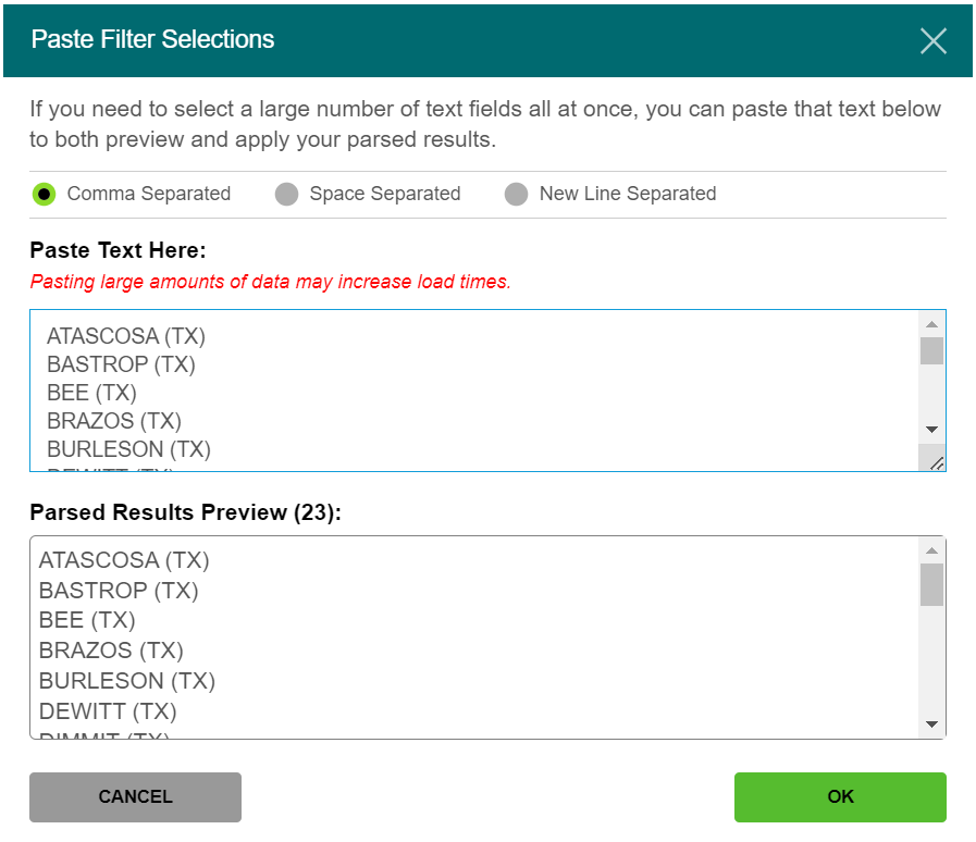
Figure 3: Pasting the Eagle Ford basin's state and county data into Drilling Info for query
1. Key takeaways
2. How are DUC wells created?
The formation of DUC wells in the oil and gas industry is caused by a variety of factors. The most straightforward reason is that they occur when operators drill more wells than they complete, and vice versa, whether by choice or not. If they drill more wells than they complete, DUC wells accumulate. If they complete more wells than they drill, DUC wells deplete. This trend can be observed in Figure 4, which showcases three distinct periods where the US DUC well counts in the seven DPR regions experienced rapid increases and decreases as a result of imbalanced drilling and completion activities.
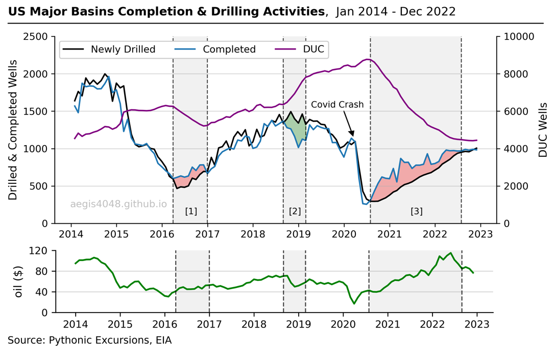
Figure 4: DUCs accumulate when drilling activity exceeds completion, and vice versa. The line plots depict three distinct periods of significant fluctuations in DUC well inventories, with [1] and [3] representing instances of rapid depletion due to high completion rates, and [2] reflecting a period of accumulation resulting from high drilling activities. WTI Crude oil prices is appended at the bottom to show the effect of commodity prices on DUCs.
Source Code For Figure (4)
import pandas as pd
import matplotlib.pyplot as plt
import numpy as np
import matplotlib.ticker as ticker

############################################# Basins ##############################################

basins = sorted(['Anadarko', 'Appalachia', 'Eagle Ford', 'Haynesville', 'Niobrara', 'Permian', 'Bakken'])

################################### DUC Wells Count per Basin #####################################

# compile a DataFrame to store count of DUC wells per basin
# source: EIA - https://www.eia.gov/petroleum/drilling/

dfs = []
for basin in basins:
    df_cur = pd.read_excel('https://aegis4048.github.io/downloads/notebooks/sample_data/Duc-EIA.xlsx', sheet_name=basin)
    df_cur['Basin'] = basin
    dfs.append(df_cur)

df = pd.concat(dfs)
df = df.sort_values('Date')
df.index = pd.to_datetime(df['Date'])

df_DUCs = df.groupby([pd.Grouper(freq='M'), 'Basin'])['DUC'].mean()
df_DUCs = df_DUCs.unstack().fillna(0)
df_DUCs = round(df_DUCs, 0)
df_DUCs['Total DUCs'] = df_DUCs.T.apply(lambda x: sum(x))

df_drilled = df.groupby([pd.Grouper(freq='M'), 'Basin'])['Drilled'].sum()
df_drilled = df_drilled.unstack().fillna(0)
df_drilled['Total Drilled'] = df_drilled.T.apply(lambda x: sum(x))

df_completed = df.groupby([pd.Grouper(freq='M'), 'Basin'])['Completed'].sum()
df_completed = df_completed.unstack().fillna(0)
df_completed['Total Completed'] = df_completed.T.apply(lambda x: sum(x))

############################################# Plot ##############################################

fig, ax = plt.subplots(figsize=(8, 4))

ax2 = ax.twinx()

ax.plot(df_drilled.index, df_drilled['Total Drilled'], color='k', label='Newly Drilled')
ax.plot(df_completed.index, df_completed['Total Completed'], label='Completed')
ax2.plot(df_DUCs.index, df_DUCs['Total DUCs'], color='purple', label='DUC')


ax.fill_between(df_drilled.index, df_drilled['Total Drilled'], df_completed['Total Completed'],
                where=(df_drilled.index >= '2016-03-1') & (df_drilled.index <= '2017-1-1'), color='red', alpha=0.4)
ax.fill_between(df_drilled.index, df_drilled['Total Drilled'], df_completed['Total Completed'],
                where=(df_drilled.index >= '2018-08-01') & (df_drilled.index <= '2019-3-1'), color='green', alpha=0.4)
ax.fill_between(df_drilled.index, df_drilled['Total Drilled'], df_completed['Total Completed'],
                where=(df_drilled.index >= '2020-07-1') & (df_drilled.index <= '2022-8-1'), color='red', alpha=0.4)

ax.axvline(x=df_drilled.index[26], color='k', linestyle='--', linewidth=1, alpha=0.7)
ax.axvline(x=df_drilled.index[35], color='k', linestyle='--', linewidth=1, alpha=0.7)
ax.axvspan(df_drilled.index[26], df_drilled.index[35], facecolor='lightgrey', alpha=0.3)

ax.axvline(x=df_drilled.index[55], color='k', linestyle='--', linewidth=1, alpha=0.7)
ax.axvline(x=df_drilled.index[61], color='k', linestyle='--', linewidth=1, alpha=0.7)
ax.axvspan(df_drilled.index[55], df_drilled.index[61], facecolor='lightgrey', alpha=0.3)

ax.axvline(x=df_drilled.index[78], color='k', linestyle='--', linewidth=1, alpha=0.7)
ax.axvline(x=df_drilled.index[102], color='k', linestyle='--', linewidth=1, alpha=0.7)
ax.axvspan(df_drilled.index[78], df_drilled.index[102], facecolor='lightgrey', alpha=0.3)

ax.set_ylim(0, 2500)
ax2.set_ylim(0, 10000)

ax.grid(axis='y', alpha=0.5)
ax.yaxis.get_major_ticks()[5].gridline.set_visible(False)
ax.spines.top.set_visible(False)
ax2.spines.top.set_visible(False)

h1, l1 = ax.get_legend_handles_labels()
h2, l2 = ax2.get_legend_handles_labels()
ax.legend(h1 + h2, l1 + l2, fontsize=10, ncol=3, loc='upper left', framealpha=1)

ax.set_ylabel('Drilled & Completed Wells', fontsize=11)
ax2.set_ylabel('DUC Wells', fontsize=11)

ax.arrow(df_drilled.index[71], 1500, 60, -270, head_width=40, head_length=60, fc='k', ec='k')
ax.text(0.58, 0.62, 'Covid Crash', fontsize=9, transform=ax.transAxes, color='k')

ax.text(0.295, 0.05, '[1]', fontsize=9, transform=ax.transAxes, color='k')
ax.text(0.53, 0.05, '[2]', fontsize=9, transform=ax.transAxes, color='k')
ax.text(0.805, 0.05, '[3]', fontsize=9, transform=ax.transAxes, color='k')

def setbold(txt):
    return ' '.join([r"$\bf{" + item + "}$" for item in txt.split(' ')])

ax.set_title(setbold('US Major Basins Completion & Drilling Activities')  + ",  Jan 2014 - Dec 2022", fontsize=12, pad=10, x=0.4, y=1.06)
ax.annotate('', xy=(-0.11, 1.07), xycoords='axes fraction', xytext=(1.11, 1.07), arrowprops=dict(arrowstyle="-", color='k'))
ax.text(0.145, 0.1, 'aegis4048.github.io', fontsize=10, ha='center', va='center',
        transform=ax.transAxes, color='grey', alpha=0.5)

fig.set_facecolor("white")
fig.tight_layout()

############################################# Plot 2 ##############################################

df = pd.read_excel('https://aegis4048.github.io/downloads/notebooks/sample_data/EIA-commodity.xls', sheet_name='Data 1')
df = df.iloc[338:-1, :-1] # between Jan 2014 to Dec 2022
df.columns = ['date', 'value']
df.reset_index(inplace=True, drop=True)
df['date'] = df['date'].apply(lambda x: x.strftime('%Y-%m'))
df['date'] = pd.to_datetime(df['date'])

fig, ax = plt.subplots(figsize=(7, 1))

ax.plot(df['date'], df['value'], color='green')

ax.set_ylabel('oil ($)', fontsize=10)
ax.set_ylim(0, 120)
ax.set_yticks(np.linspace(0, 120, 4))
ax.tick_params(axis='both', which='major', labelsize=9)

ax.axvspan(df_drilled.index[26], df_drilled.index[35], facecolor='lightgrey', alpha=0.3)
ax.axvspan(df_drilled.index[55], df_drilled.index[61], facecolor='lightgrey', alpha=0.3)
ax.axvspan(df_drilled.index[78], df_drilled.index[103], facecolor='lightgrey', alpha=0.3)

ax.axvline(x=df_drilled.index[26], color='k', linestyle='--', linewidth=1, alpha=0.7)
ax.axvline(x=df_drilled.index[35], color='k', linestyle='--', linewidth=1, alpha=0.7)
ax.axvline(x=df_drilled.index[55], color='k', linestyle='--', linewidth=1, alpha=0.7)
ax.axvline(x=df_drilled.index[61], color='k', linestyle='--', linewidth=1, alpha=0.7)
ax.axvline(x=df_drilled.index[78], color='k', linestyle='--', linewidth=1, alpha=0.7)
ax.axvline(x=df_drilled.index[103], color='k', linestyle='--', linewidth=1, alpha=0.7)

ax.grid(axis='y', alpha=0.5)
ax.spines['right'].set_visible(False)
ax.spines['top'].set_visible(False)
ax.yaxis.get_major_ticks()[-1].gridline.set_visible(False)

ax.annotate('Source: Pythonic Excursions, EIA', xy=(-0.11, -.5), xycoords='axes fraction', fontsize=9)
Here I list more detailed reasons as to why operators may choose to not complete their well.
Cost efficiency with batch-fracking or batch-drilling
As an efficient operator, it is ideal to avoid engaging a fracturing fleet until all logistical requirements have been thoroughly understood and procured and a substantial number of wells have been collected for prolonged, uninterrupted operations. This can be achieved either by maintaining a consistent inventory of wells waiting to be completed or by alternating the company's focus in the region between drilling a series of wells and then completing them all. If there are 10 wells in one location and it takes 10 days to drill each well, the first drilled well will stay idle for at least 90 days before it can be completed. This lag can result in the formation of additional DUC wells in the event of an unforeseen circumstance that renders fracturing unfeasible or undesirable.
Drilling contracts that are too expensive to revoke
Often times the drilling contracts between an operator and a service company entails drilling a batch of wells and expensive contract revokation fee. If the oil price suddenly drops while drilling the contracted batch of wells, the operator may choose not to complete the drilled wells while letting the rig crews keep drilling new wells due to the existing contract. This was the most apparent in the recent COVID crash, which took place around March of 2020. Taking a close look at Figure 4 around March of 2020 (slightly to the left of [3]), one can observe that there higher drilling than completion activities, which temporarily boosted the number of DUCs until July of 2020 (start of [3]). This happened because there were rig contracts that were still in effect few months after the COVID crash. However, this phenomena did not last long once those contracts expired or have been fulfilled, thus rapidly depleting the number of DUCs until late 2022.
Constraints on capital spending
The operator may choose not to finish their wells due to restrictions on the company's capital expenditures or adverse market circumstances, opting instead to wait for better economics. However, this approach may not always be advisable, as DUC wells older than two years have a low probability, less than 5%, of being completed due to issues such as lost leases.
Lack of infrastructure
An operator may leave a well uncompleted if there is no nearby pipeline to transport the produced gas after a pad site is cleared and a well is drilled. However, unexpected issues during pipeline construction may result in the well remaining as a DUC well for an extended period until resolved.
3. DUC wells and economic complications
DUC wells are a form of hydrocarbon storage under the ground instead of on the surface storage facilities. The operators invest on drilling first and take profits later when its desirable. This unique characteristics of DUCs create economic complications for the oil and gas industry due to the following reasons:
Timing: DUC wells are partially completed sources of supply that can be brought to market more quickly and at a lower cost than a newly drilled well. However, completing DUC wells at the right time to balance the market demand for energy can be challenging.
Market fluctuations: DUC wells are often used to keep up with demand during times of high energy demand. However, during periods of declining oil prices, completing DUC wells may not be economically viable, leading to a buildup of uncompleted wells. This has been the most apparent between late 2018 to early 2019; WTI crude dropped from
$
86 to$
54. This accumulation of DUCs due to oil price drop can be observed in Figure 4's highlighted area [2].
Rig contracts: In times of declining oil prices, operators may continue to drill wells due to rig contracts, but not complete these wells and bring them into production. This can result in a buildup of DUC wells that may not be economically viable to complete in the future (due to reasons like lost leases).
Profit-taking: Completing DUC wells is essentially a profit-taking process done on wells with substantial investment already made. However, if the timing of completion is not aligned with market demand or if capital is not available, the profit-taking process may not yield the expected results.
Capital management: The inventory levels of DUC wells are closely linked to the availability of industry capital. When capital is abundant, producers tend to increase drilling relative to completions, leading to a rise in DUC inventory. On the other hand, when capital is scarce, producers prioritize well completion over new drilling, which can lead to a depletion of DUC wells.
3.1. Potential depletion of DUC wells and enegy supply shortage
The COVID-19 pandemic resulted in a reduction of available capital for the oil and gas industry. To conserve cash, many operators prioritized well completion over new drilling, enabling them to maintain production with less capital. However, this strategy of profit-taking cannot be sustained in the long-term and resulted in a rapid decrease of DUC wells in the US, raising concerns about the potential depletion of DUCs and energy supply shortages.
Figure 5 demonstrates the swift depletion rate of DUCs since July 2020. If this rate continued, the US oil and gas industry would have exhausted its DUC wells by the end of 2023, potentially leading to an energy shortage. Fortunately, drilling activity caught up with completion activities by mid-2022, resulting in a stable level of DUC wells now.
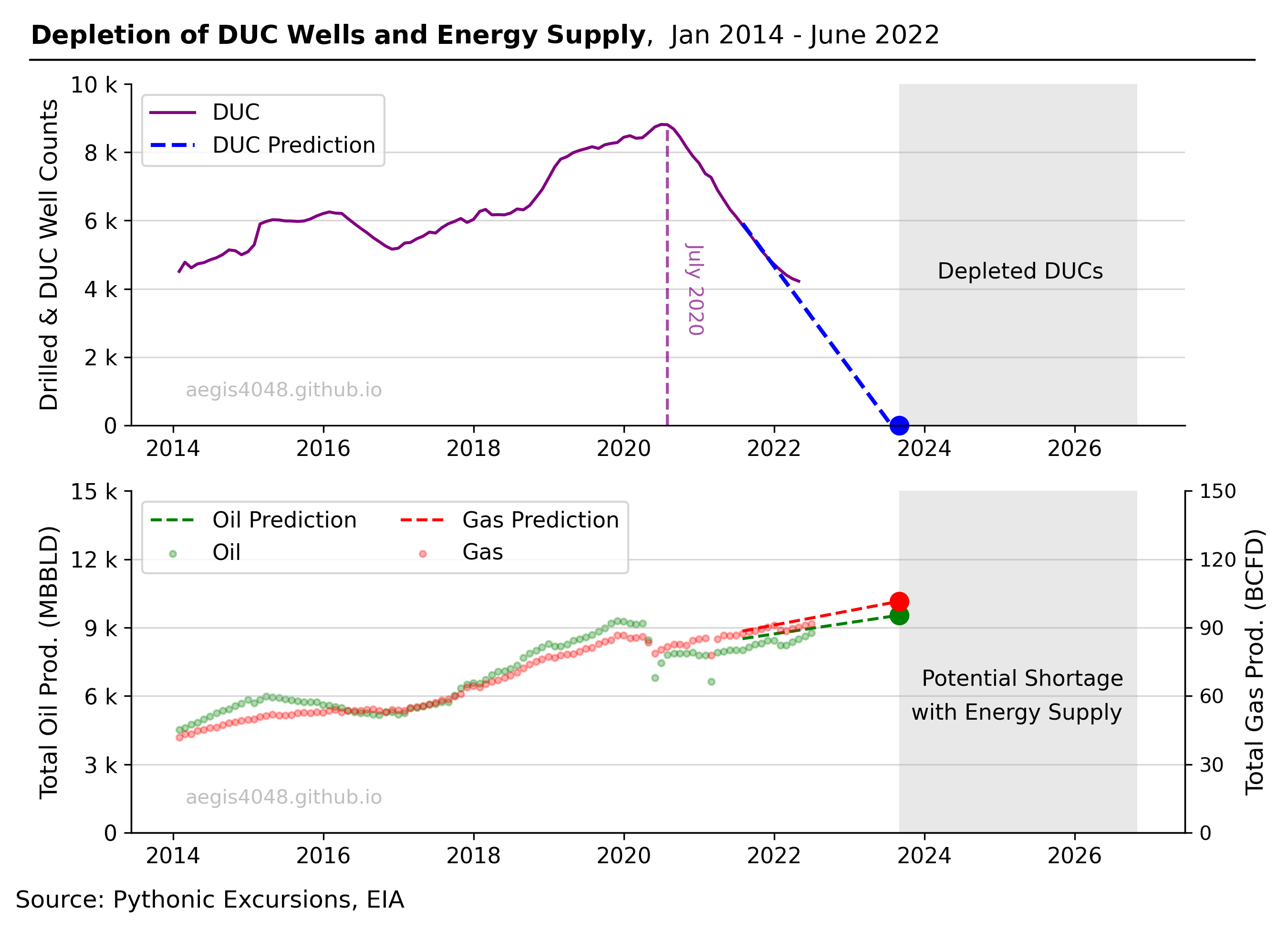
Figure 5: Rapid depletion of US DUC wells since July 2020. Prolonged depletion of DUC wells may result in potential shortage with energy supply if the operators don't drill more wells.
Source Code For Figure (5)
import pandas as pd
import matplotlib.pyplot as plt
import numpy as np
import matplotlib.ticker as ticker
from sklearn import linear_model
import datetime

############################################# Basins ##############################################

basins = sorted(['Anadarko', 'Appalachia', 'Eagle Ford', 'Haynesville', 'Niobrara', 'Permian', 'Bakken'])

################################### DUC Wells Count per Basin #####################################

# compile a DataFrame to store count of DUC wells per basin
# source: EIA - https://www.eia.gov/petroleum/drilling/

dfs = []
for basin in basins:
    df_cur = pd.read_excel('https://aegis4048.github.io/downloads/notebooks/sample_data/Duc-EIA-old.xlsx', sheet_name=basin)
    df_cur['Basin'] = basin
    dfs.append(df_cur)

df = pd.concat(dfs)
df = df.sort_values('Date')
df.index = pd.to_datetime(df['Date'])

df_DUCs = df.groupby([pd.Grouper(freq='M'), 'Basin'])['DUC'].mean()
df_DUCs = df_DUCs.unstack().fillna(0)
df_DUCs = round(df_DUCs, 0)
df_DUCs['Total DUCs'] = df_DUCs.T.apply(lambda x: sum(x))

df_drilled = df.groupby([pd.Grouper(freq='M'), 'Basin'])['Drilled'].sum()
df_drilled = df_drilled.unstack().fillna(0)
df_drilled['Total Drilled'] = df_drilled.T.apply(lambda x: sum(x))

df_completed = df.groupby([pd.Grouper(freq='M'), 'Basin'])['Completed'].sum()
df_completed = df_completed.unstack().fillna(0)
df_completed['Total Completed'] = df_completed.T.apply(lambda x: sum(x))

#################### Import All Data - Rig Count, Oil & Gas Prod per Basins #######################

dfs2 = []
for basin in basins:
    df_cur = pd.read_excel('https://aegis4048.github.io/downloads/notebooks/sample_data/dpr-data-old.xlsx', sheet_name=basin + ' Region', skiprows=1)
    df_cur['Basin'] = basin
    dfs2.append(df_cur)

year_cutoff = '2013' # counting from year_cutoff + 1
date_header = 'Month'

df2 = pd.concat(dfs2)
df2 = df2.sort_values(date_header)
df2.index = pd.to_datetime(df2[date_header])
df2.drop(df2.columns[[2, 3, 5, 6]], axis=1, inplace=True)
df2.columns = ['Date', 'Rig Count', 'Total Oil Prod (BBLD)', 'Total Gas Prod (MCFD)', 'Basin']
df2 = df2[df2.index > year_cutoff + '-12-31']

# current year (2022) prediction parameter
num_month_2022 = 6 # number of months in data set for current year
pred_factor = 12 / num_month_2022

################################ Cross Table for Gas Production ###################################

# Total Gas Production
df2_total_gas_prod = df2.groupby([pd.Grouper(freq='M'), 'Basin'])['Total Gas Prod (MCFD)'].sum()
df2_total_gas_prod = df2_total_gas_prod.unstack().fillna(0)
df2_total_gas_prod['Total Gas (BCFD)'] = df2_total_gas_prod.T.apply(lambda x: sum(x))
df2_total_gas_prod = df2_total_gas_prod / 1000000

################################ Cross Table for Oil Production ###################################

df2_total_oil_prod = df2.groupby([pd.Grouper(freq='M'), 'Basin'])['Total Oil Prod (BBLD)'].sum()
df2_total_oil_prod = df2_total_oil_prod.unstack().fillna(0)
df2_total_oil_prod['Total Oil (MBBLD)'] = df2_total_oil_prod.T.apply(lambda x: sum(x))
df2_total_oil_prod = df2_total_oil_prod / 1000

############################################# Plot ##############################################

axis_label_fontsize = 12
title_fontsize = 13
legend_fontsize = 11

fig, axes = plt.subplots(2, 1, figsize=(9, 6.5))

ax1 = axes[0]
ax2 = axes[1]
ax3 = ax2.twinx()

n = 16

# extends the right-end of the x-axis
ext = 38
x_extender = df_DUCs.index.union(df_DUCs.index.shift(n + ext)[-(n + ext):])
x_extender_y = [1 for item in x_extender]

ax1.plot(x_extender, x_extender_y, alpha=0)
ax2.plot(x_extender, x_extender_y, alpha=0)

ax1.axvspan(x_extender[-ext-1], x_extender[-1], facecolor='lightgrey', alpha=0.5)
ax2.axvspan(x_extender[-ext-1], x_extender[-1], facecolor='lightgrey', alpha=0.5)

################################### DUC Wells Linear Regression ###################################

X_pred_plot = df_DUCs.index.union(df_DUCs.index.shift(n)[-n:])
X_pred = X_pred_plot.to_julian_date().values.reshape(-1, 1)

X = df_DUCs.index.to_julian_date().values.reshape(-1, 1)
y = df_DUCs['Total DUCs'].values

fit_begin = 79
fit_end = -3
plot_begin = 90

ols = linear_model.LinearRegression()
model = ols.fit(X[fit_begin: fit_end], y[fit_begin: fit_end])
response = model.predict(X_pred[plot_begin:])

ax1.plot(df_DUCs.index, df_DUCs['Total DUCs'], color='purple', label='DUC')
ax1.plot(X_pred_plot[plot_begin:], response, color='b', label='DUC Prediction', linestyle='--', linewidth=2)
ax1.vlines(x=df_DUCs.index[fit_begin - 1], ymin=0, ymax=max(y) - 100, color='purple', alpha=0.7, linestyle='--')
ax1.scatter(X_pred_plot[-1], 0, marker='o', color='b', label='point', clip_on=False, s=80)

############################# Oil and Gas Production Linear Regression ############################

n = n - 2
X_pred_plot = df2_total_oil_prod.index.union(df2_total_oil_prod.index.shift(n)[-n:])
X_pred = X_pred_plot.to_julian_date().values.reshape(-1, 1)

X = df2_total_oil_prod.index.to_julian_date().values.reshape(-1, 1)

y_oil = df2_total_oil_prod['Total Oil (MBBLD)'].values
y_gas = df2_total_gas_prod['Total Gas (BCFD)'].values

ols_oil = linear_model.LinearRegression()
ols_gas = linear_model.LinearRegression()
model_oil = ols_oil.fit(X, y_oil)
model_gas = ols_gas.fit(X, y_gas)
response_oil = model_oil.predict(X_pred)
response_gas = model_gas.predict(X_pred)

ax2.plot(X_pred_plot[plot_begin:], response_oil[plot_begin:], label='Oil Prediction', color='green', linestyle='--')
ax3.plot(X_pred_plot[plot_begin:], response_gas[plot_begin:], label='Gas Prediction', color='red', linestyle='--')

ax2.scatter(X_pred_plot[-1], response_oil[-1], marker='o', color='green', clip_on=False, s=80)
ax3.scatter(X_pred_plot[-1], response_gas[-1], marker='o', color='red', clip_on=False, s=80)

ax2.scatter(df2_total_oil_prod.index, df2_total_oil_prod['Total Oil (MBBLD)'], label='Oil', marker='o', color='green', s=10, alpha=0.3)
ax3.scatter(df2_total_gas_prod.index, df2_total_gas_prod['Total Gas (BCFD)'], label='Gas', marker='o', color='red', s=10, alpha=0.3)

ax1.set_ylim(0, 10000)
ax2.set_ylim(0, 15000)
ax3.set_ylim(0, 150)

ax1.set_ylabel('Drilled & DUC Well Counts', fontsize=axis_label_fontsize)
ax2.set_ylabel('Total Oil Prod. (MBBLD)', fontsize=axis_label_fontsize)
ax2.set_yticks(np.arange(0, 15001, 3000))
ax3.set_ylabel('Total Gas Prod. (BCFD)', fontsize=axis_label_fontsize)
ax3.set_yticks(np.arange(0, 151, 30))

ax1.tick_params(axis='both', which='major', labelsize=11)
ax2.tick_params(axis='both', which='major', labelsize=11)

ax1.grid(axis='y', alpha=0.5)
ax1.yaxis.get_major_ticks()[5].gridline.set_visible(False)
ax2.grid(axis='y', alpha=0.5)
ax2.yaxis.get_major_ticks()[5].gridline.set_visible(False)

ax1.spines.top.set_visible(False)
ax1.spines.right.set_visible(False)
ax2.spines.top.set_visible(False)
ax3.spines.top.set_visible(False)

h1, l1 = ax1.get_legend_handles_labels()
ax1.legend(h1[:2], l1[:2], loc='upper left', fontsize=legend_fontsize)
h2, l2 = ax2.get_legend_handles_labels()
h3, l3 = ax3.get_legend_handles_labels()
ax2.legend(h2 + h3, l2 + l3, fontsize=legend_fontsize, ncol=2, loc='upper left')

ax1.yaxis.set_major_formatter(ticker.EngFormatter())
ax2.yaxis.set_major_formatter(ticker.EngFormatter())
ax3.yaxis.set_major_formatter(ticker.EngFormatter())

def setbold(txt):
    return ' '.join([r"$\bf{" + item + "}$" for item in txt.split(' ')])

ax1.set_title(setbold('Depletion of DUC Wells and Energy Supply')  + ",  Jan 2014 - June 2022",
             fontsize=title_fontsize, pad=10, x=0.335, y=1.06)
ax1.annotate('', xy=(-0.1, 1.07), xycoords='axes fraction', xytext=(1.07, 1.07), arrowprops=dict(arrowstyle="-", color='k'))
ax1.text(0.535, 0.4, 'July 2020', fontsize=10, ha='center', va='center',
        transform=ax1.transAxes, color='purple', alpha=0.7, rotation=270)

ax2.annotate('Source: Pythonic Excursions, EIA', xy=(-0.11, -0.22), xycoords='axes fraction', fontsize=12)
ax1.text(0.145, 0.1, 'aegis4048.github.io', fontsize=10, ha='center', va='center',
        transform=ax1.transAxes, color='grey', alpha=0.5)
ax2.text(0.145, 0.1, 'aegis4048.github.io', fontsize=10, ha='center', va='center',
        transform=ax2.transAxes, color='grey', alpha=0.5)

ax1.text(0.765, 0.43, 'Depleted DUCs', fontsize=11, transform=ax1.transAxes, color='k')
ax2.text(0.75, 0.43, 'Potential Shortage', fontsize=11, transform=ax2.transAxes, color='k')
ax2.text(0.74, 0.33, 'with Energy Supply', fontsize=11, transform=ax2.transAxes, color='k')

fig.set_facecolor("white")
fig.tight_layout()
3.2. Recent trend: more production with less drilling
Some readers may recall President Biden's request for the US oil and gas industry to ramp up drilling in order to curb the recent surge in gasoline prices. The industry reportedly hesitated to comply due to pressure from Wall Street for immediate financial returns. However, this is not the sole reason for the industry's reluctance to return to their previous drilling levels from 2014. Advances in technology (specifically horizontal drilling) have enabled the industry to produce more oil and gas with fewer wells, meaning they no longer need to drill as many wells as in the past to meet production demands.
Figure 6 highlights three key points that demonstrate a clear trend. The decline in the number of drilling operations can be observed at [1], [2], and [3], while production steadily increases. A comparison to July 2018 [2] shows a 31% reduction in the number of newly drilled wells, but a 26% increase in oil production and a 35% increase in gas production. The contrast becomes even more striking when compared to September 2014 [1], where drilling activity decreased by 50% while production of both oil and gas nearly doubled.
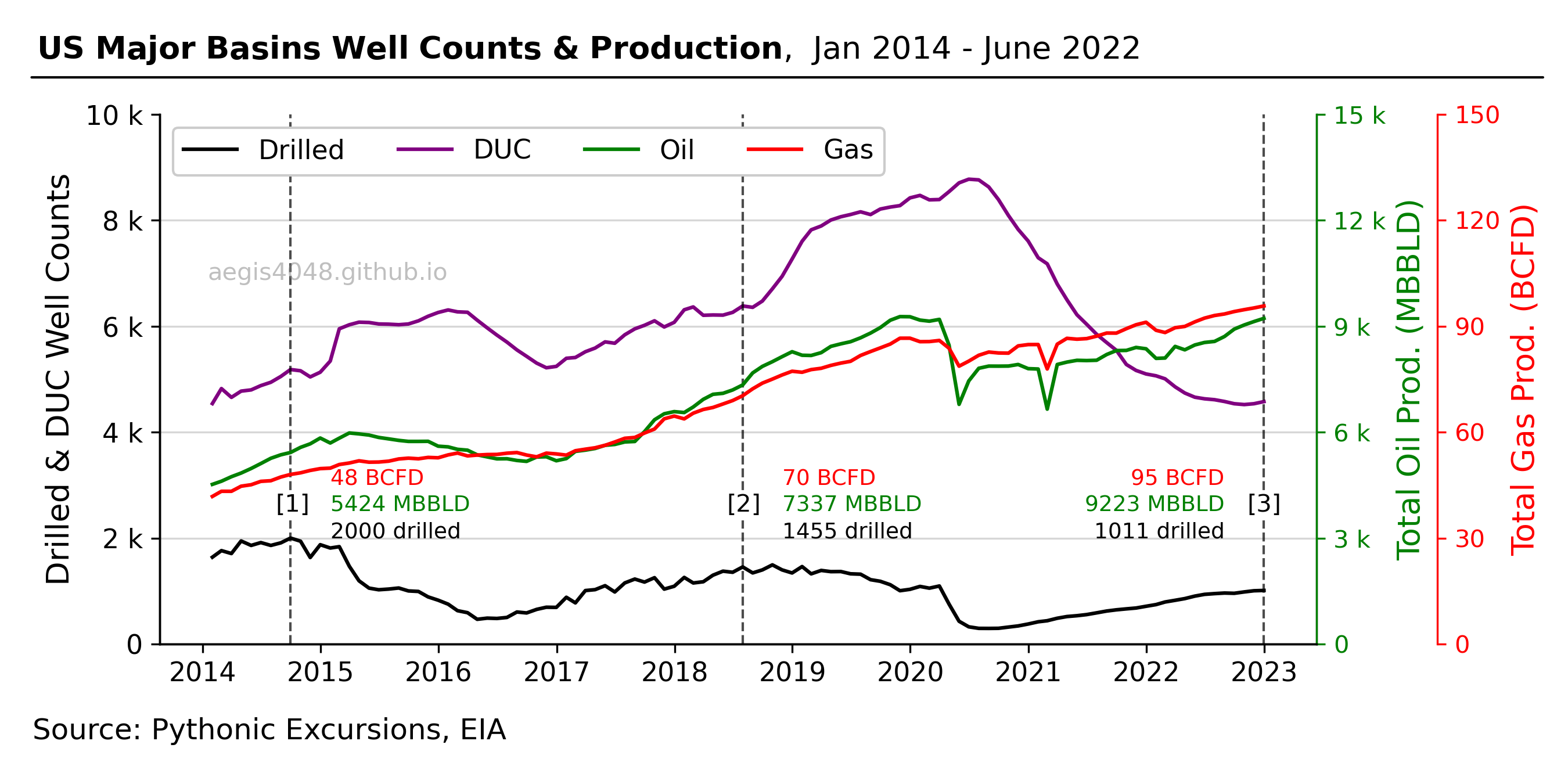
Figure 6: Recent trend in production and drilling activities and count of DUC wells. We've been producing more oil and gas with less drilling activities over time.
Source Code For Figure (6)
import pandas as pd
import matplotlib.pyplot as plt
import numpy as np
import matplotlib.ticker as ticker

############################################# Basins ##############################################

basins = sorted(['Anadarko', 'Appalachia', 'Eagle Ford', 'Haynesville', 'Niobrara', 'Permian', 'Bakken'])

################################### DUC Wells Count per Basin #####################################

# compile a DataFrame to store count of DUC wells per basin
# source: EIA - https://www.eia.gov/petroleum/drilling/

dfs = []
for basin in basins:
    df_cur = pd.read_excel('https://aegis4048.github.io/downloads/notebooks/sample_data/Duc-EIA.xlsx', sheet_name=basin)
    df_cur['Basin'] = basin
    dfs.append(df_cur)

df = pd.concat(dfs)
df = df.sort_values('Date')
df.index = pd.to_datetime(df['Date'])

df_DUCs = df.groupby([pd.Grouper(freq='M'), 'Basin'])['DUC'].mean()
df_DUCs = df_DUCs.unstack().fillna(0)
df_DUCs = round(df_DUCs, 0)
df_DUCs['Total DUCs'] = df_DUCs.T.apply(lambda x: sum(x))

df_drilled = df.groupby([pd.Grouper(freq='M'), 'Basin'])['Drilled'].sum()
df_drilled = df_drilled.unstack().fillna(0)
df_drilled['Total Drilled'] = df_drilled.T.apply(lambda x: sum(x))

df_completed = df.groupby([pd.Grouper(freq='M'), 'Basin'])['Completed'].sum()
df_completed = df_completed.unstack().fillna(0)
df_completed['Total Completed'] = df_completed.T.apply(lambda x: sum(x))

#################### Import All Data - Rig Count, Oil & Gas Prod per Basins #######################

dfs2 = []
for basin in basins:
    df_cur = pd.read_excel('https://aegis4048.github.io/downloads/notebooks/sample_data/dpr-data.xlsx', sheet_name=basin + ' Region', skiprows=1)
    df_cur['Basin'] = basin
    dfs2.append(df_cur)

year_cutoff = '2013' # counting from year_cutoff + 1
date_header = 'Month'

df2 = pd.concat(dfs2)
df2 = df2.sort_values(date_header)
df2.index = pd.to_datetime(df2[date_header])
df2.drop(df2.columns[[2, 3, 5, 6]], axis=1, inplace=True)
df2.columns = ['Date', 'Rig Count', 'Total Oil Prod (BBLD)', 'Total Gas Prod (MCFD)', 'Basin']
df2 = df2[df2.index > year_cutoff + '-12-31']

# current year (2022) prediction parameter
num_month_2022 = 6 # number of months in data set for current year
pred_factor = 12 / num_month_2022

################################ Cross Table for Gas Production ###################################

# Total Gas Production
df2_total_gas_prod = df2.groupby([pd.Grouper(freq='M'), 'Basin'])['Total Gas Prod (MCFD)'].sum()
df2_total_gas_prod = df2_total_gas_prod.unstack().fillna(0)
df2_total_gas_prod['Total Gas (BCFD)'] = df2_total_gas_prod.T.apply(lambda x: sum(x))
df2_total_gas_prod = df2_total_gas_prod / 1000000

################################ Cross Table for Oil Production ###################################

df2_total_oil_prod = df2.groupby([pd.Grouper(freq='M'), 'Basin'])['Total Oil Prod (BBLD)'].sum()
df2_total_oil_prod = df2_total_oil_prod.unstack().fillna(0)
df2_total_oil_prod['Total Oil (MBBLD)'] = df2_total_oil_prod.T.apply(lambda x: sum(x))
df2_total_oil_prod = df2_total_oil_prod / 1000

############################################# Plot ##############################################

axis_label_fontsize = 13
title_fontsize = 13
legend_fontsize = 11

fig, ax = plt.subplots(figsize=(9, 4.5))

ax3 = ax.twinx()
ax4 = ax.twinx()

ax.plot(df_drilled.index, df_drilled['Total Drilled'], color='k', label='Drilled')
ax.plot(df_DUCs.index, df_DUCs['Total DUCs'], color='purple', label='DUC')
ax3.plot(df2_total_oil_prod.index, df2_total_oil_prod['Total Oil (MBBLD)'], label='Oil', color='green')
ax4.plot(df2_total_gas_prod.index, df2_total_gas_prod['Total Gas (BCFD)'], label='Gas', color='red')

ax.set_ylim(0, 10000)
ax3.set_ylim(0, 15000)
ax4.set_ylim(0, 150)

ax.set_ylabel('Drilled & DUC Well Counts', fontsize=axis_label_fontsize)

ax3.tick_params(axis='y', colors='green')
#ax3.spines['right'].set_position(('outward', 50))
ax3.spines['right'].set_color('green')
ax3.set_ylabel('Total Oil Prod. (MBBLD)', color='green', fontsize=axis_label_fontsize)
ax3.set_yticks(np.arange(0, 15001, 3000))

ax4.tick_params(axis='y', colors='red')
ax4.spines['right'].set_position(('outward', 50))
ax4.spines['right'].set_color('red')
ax4.set_ylabel('Total Gas Prod. (BCFD)', color='red', fontsize=axis_label_fontsize)
ax4.set_yticks(np.arange(0, 151, 30))
ax.tick_params(axis='both', which='major', labelsize=11)

ax.grid(axis='y', alpha=0.5)
ax.yaxis.get_major_ticks()[5].gridline.set_visible(False)

ax.spines.top.set_visible(False)
ax3.spines.top.set_visible(False)
ax4.spines.top.set_visible(False)

h1, l1 = ax.get_legend_handles_labels()
h3, l3 = ax3.get_legend_handles_labels()
h4, l4 = ax4.get_legend_handles_labels()
ax.legend(h1 + h3 + h4, l1 + l3 + l4, fontsize=legend_fontsize, ncol=4, loc='upper left', framealpha=1)

ax.yaxis.set_major_formatter(ticker.EngFormatter())
ax3.yaxis.set_major_formatter(ticker.EngFormatter())
ax4.yaxis.set_major_formatter(ticker.EngFormatter())

def setbold(txt):
    return ' '.join([r"$\bf{" + item + "}$" for item in txt.split(' ')])

ax.set_title(setbold('US Major Basins Well Counts & Production')  + ",  Jan 2014 - June 2022",
             fontsize=title_fontsize, pad=10, x=0.37, y=1.06)
ax.annotate('', xy=(-0.115, 1.07), xycoords='axes fraction', xytext=(1.2, 1.07), arrowprops=dict(arrowstyle="-", color='k'))
ax.annotate('Source: Pythonic Excursions, EIA', xy=(-0.11, -0.18), xycoords='axes fraction', fontsize=12)
ax.text(0.145, 0.7, 'aegis4048.github.io', fontsize=10, ha='center', va='center',
        transform=ax.transAxes, color='grey', alpha=0.5)

ax.axvline(x=df_drilled.index[8], color='k', linestyle='--', linewidth=1, alpha=0.7)
ax.axvline(x=df_drilled.index[54], color='k', linestyle='--', linewidth=1, alpha=0.7)
ax.axvline(x=df_drilled.index[-1], color='k', linestyle='--', linewidth=1, alpha=0.7)

t1 = ax.text(0.1, 0.25, '[1]', fontsize=10, transform=ax.transAxes, color='k', )
t2 = ax.text(0.49, 0.25, '[2]', fontsize=10, transform=ax.transAxes, color='k')
t3 = ax.text(0.94, 0.25, '[3]', fontsize=10, transform=ax.transAxes, color='k')

t1.set_bbox(dict(facecolor='white', alpha=1, edgecolor='white', pad=1))
t2.set_bbox(dict(facecolor='white', alpha=1, edgecolor='white', pad=1))
t3.set_bbox(dict(facecolor='white', alpha=1, edgecolor='white', pad=1))

oil1 = str(int(df2_total_oil_prod['Total Oil (MBBLD)'][8])) + ' MBBLD'
gas1 = str(int(df2_total_gas_prod['Total Gas (BCFD)'][8])) + ' BCFD'
drill1 = str(int(df_drilled['Total Drilled'][8])) + ' drilled'
ax.text(df_drilled.index[8 + 4], 2500, oil1, fontsize=9, color='green', bbox=dict(facecolor='none', edgecolor='none'))
ax.text(df_drilled.index[8 + 4], 3000, gas1, fontsize=9, color='red', bbox=dict(facecolor='none', edgecolor='none'))
ax.text(df_drilled.index[8 + 4], 2000, drill1, fontsize=9, color='k', bbox=dict(facecolor='none', edgecolor='none'))


oil2 = str(int(df2_total_oil_prod['Total Oil (MBBLD)'][54])) + ' MBBLD'
gas2 = str(int(df2_total_gas_prod['Total Gas (BCFD)'][54])) + ' BCFD'
drill2 = str(int(df_drilled['Total Drilled'][54])) + ' drilled'
ax.text(df_drilled.index[54 + 4], 2500, oil2, fontsize=9, color='green', bbox=dict(facecolor='none', edgecolor='none'))
ax.text(df_drilled.index[54 + 4], 3000, gas2, fontsize=9, color='red', bbox=dict(facecolor='none', edgecolor='none'))
ax.text(df_drilled.index[54 + 4], 2000, drill2, fontsize=9, color='k', bbox=dict(facecolor='none', edgecolor='none'))

ha = 'right'
oil3 = str(int(df2_total_oil_prod['Total Oil (MBBLD)'][-1])) + ' MBBLD'
gas3 = str(int(df2_total_gas_prod['Total Gas (BCFD)'][-1])) + ' BCFD'
drill3 = str(int(df_drilled['Total Drilled'][-1])) + ' drilled'
ax.text(df_drilled.index[-1 - 4], 2500, oil3, fontsize=9, color='green', ha=ha, bbox=dict(facecolor='none', edgecolor='none'))
ax.text(df_drilled.index[-1 - 4], 3000, gas3, fontsize=9, color='red', ha=ha, bbox=dict(facecolor='none', edgecolor='none'))
ax.text(df_drilled.index[-1 - 4], 2000, drill3, fontsize=9, color='k', ha=ha, bbox=dict(facecolor='none', edgecolor='none'))

fig.set_facecolor("white")
fig.tight_layout()
The improvement in production efficiency despite the reduction in drilling can be attributed to the increasing use of horizontal wells. As compared to vertical wells, horizontal wells produce 2.5 to 7 times more, allowing the industry to meet demand with fewer drilling operations. As illustrated in Figure 7, during economic downturns, the industry has favored horizontal wells by significantly reducing the number of vertical wells. It demonstrates a steady decrease in vertical wells, indicating that the majority of modern day drilling operations now consist of 91% horizontal wells and only 9% vertical wells.
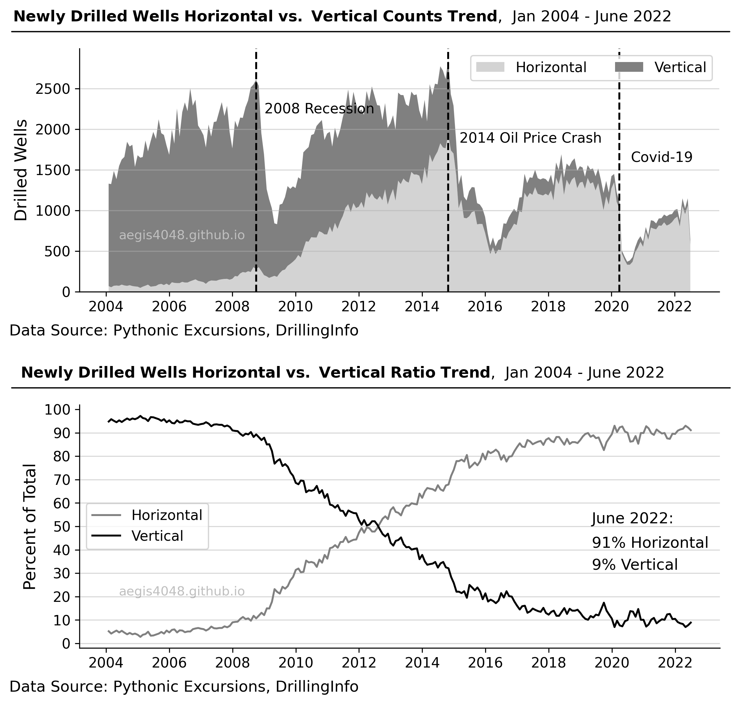
Figure 7: Historically the US oil and gas industry has turned into horizontal drilling during the times of economic crisis. Modern day drilling is mostly horizontal wells, which explains the higher production rates despite low drilling activities compared to 2014.
Source Code For Figure (7)
import pandas as pd
import numpy as np
import matplotlib.pyplot as plt
import seaborn as sns
from matplotlib.colors import LinearSegmentedColormap
import matplotlib.ticker as ticker
import warnings

############################################# Basins ##############################################

basins = sorted(['Anadarko', 'Appalachia', 'Eagle Ford', 'Haynesville', 'Niobrara', 'Permian', 'Bakken'])

################################# Drilled Wells Count per Basin ###################################

# import multiple csv files of basins and compile them into yearly count sum
# source: DrillingInfo

filename = 'https://aegis4048.github.io/downloads/notebooks/sample_data/Drill_Type_2004.xlsx'

# suppress warnings
warnings.filterwarnings('ignore')
warnings.simplefilter('ignore')

dfs = []
for basin in basins:
    df = pd.read_excel(filename, sheet_name=basin)
    df = df[df['Spud Date'].notna()]
    df['Basin'] = basin
    df['Year'] = df['Spud Date'].apply(lambda x: str(x).split('-')[0])
    dfs.append(df)

df_drilltype = pd.concat(dfs)
df_drilltype = df_drilltype.sort_values('Spud Date')
df_drilltype.index = pd.to_datetime(df_drilltype['Spud Date'])

df_drilltype = df_drilltype.groupby(pd.Grouper(freq='M'))['Drill Type'].value_counts(sort=True)
df_drilltype = df_drilltype.unstack().fillna(0).drop(['D', 'U'], axis=1)

df_drilltype_percent = df_drilltype.apply(lambda x: round(x / x.sum() * 100, 2), axis=1)
df_drilltype_percent = round(df_drilltype_percent, 1)

############################################# Plot ##############################################

fig, ax = plt.subplots(figsize=(8, 4))

x = df_drilltype.index
y = np.array([df_drilltype['H'].values, df_drilltype['V'].values])

ax.stackplot(x, *y, labels=['Horizontal', 'Vertical'], colors=['lightgrey', 'grey'])
ax.set_ylabel('Drilled Wells', fontsize=13)
ax.axvline(x=df_drilltype.index[-93], color='k', linestyle='--')
ax.axvline(x=df_drilltype.index[-28], color='k', linestyle='--')
ax.axvline(x=df_drilltype.index[-166], color='k', linestyle='--')

ax.grid(axis='y', alpha=0.5)
ax.yaxis.get_major_ticks()[6].gridline.set_visible(False)
ax.spines.top.set_visible(False)
ax.spines.right.set_visible(False)

ax.legend(fontsize=11, ncol=3, loc='upper right')
ax.tick_params(axis='both', which='major', labelsize=11)

def setbold(txt):
    return ' '.join([r"$\bf{" + item + "}$" for item in txt.split(' ')])

ax.set_title(setbold('Newly Drilled Wells Horizontal vs. Vertical Counts Trend')  + ",  Jan 2004 - June 2022", fontsize=12, pad=10, x=0.41, y=1.06)
ax.annotate('', xy=(-0.11, 1.07), xycoords='axes fraction', xytext=(1.02, 1.07), arrowprops=dict(arrowstyle="-", color='k'))
ax.annotate('Data Source: Pythonic Excursions, DrillingInfo', xy=(-0.11, -0.18), xycoords='axes fraction', fontsize=12)
ax.text(0.16, 0.23, 'aegis4048.github.io', fontsize=10, ha='center', va='center',
        transform=ax.transAxes, color='white', alpha=0.5)
ax.text(0.705, 0.63, '2014 Oil Price Crash', fontsize=11, ha='center', va='center',
        transform=ax.transAxes, color='k')
ax.text(0.91, 0.55, 'Covid-19', fontsize=11, ha='center', va='center',
        transform=ax.transAxes, color='k')
ax.text(0.375, 0.75, '2008 Recession', fontsize=11, ha='center', va='center',
        transform=ax.transAxes, color='k')

fig.set_facecolor("white")
fig.tight_layout()


#################################################################################################

fig, ax = plt.subplots(figsize=(8, 4))

ax.plot(df_drilltype_percent.index, df_drilltype_percent['H'], color='grey', label='Horizontal')
ax.plot(df_drilltype_percent.index, df_drilltype_percent['V'], color='k', label='Vertical')
ax.set_ylabel('Percent of Total', fontsize=13)
ax.tick_params(axis='both', which='major', labelsize=11)
ax.set_yticks(np.arange(0, 101, 10))

ax.grid(axis='y', alpha=0.5)
ax.yaxis.get_major_ticks()[10].gridline.set_visible(False)
ax.spines.top.set_visible(False)
ax.spines.right.set_visible(False)

ax.legend(fontsize=11, loc='center left')

def setbold(txt):
    return ' '.join([r"$\bf{" + item + "}$" for item in txt.split(' ')])

ax.set_title(setbold('Newly Drilled Wells Horizontal vs. Vertical Ratio Trend')  + ",  Jan 2004 - June 2022", fontsize=12, pad=10, x=0.41, y=1.06)
ax.annotate('', xy=(-0.11, 1.07), xycoords='axes fraction', xytext=(1.02, 1.07), arrowprops=dict(arrowstyle="-", color='k'))
ax.annotate('Data Source: Pythonic Excursions, DrillingInfo', xy=(-0.11, -0.18), xycoords='axes fraction', fontsize=12)
ax.text(0.16, 0.23, 'aegis4048.github.io', fontsize=10, ha='center', va='center',
        transform=ax.transAxes, color='grey', alpha=0.5)
ax.text(0.8, 0.43, '91% Horizontal', fontsize=12, ha='left', va='center',
        transform=ax.transAxes, color='k')
ax.text(0.8, 0.34, '9% Vertical', fontsize=12, ha='left', va='center',
        transform=ax.transAxes, color='k')
ax.text(0.8, 0.53, 'June 2022:', fontsize=12, ha='left', va='center',
        transform=ax.transAxes, color='k')

fig.set_facecolor("white")
fig.tight_layout()
4. Continued discussion: "Dead" DUC wells
DUC wells are considered to be a working oil field capital because the wells can be turned on line for production for cheap. However, the empirical evidences suggests that the DUC wells may no longer function as a working capital if completion is delayed for too long. The empirical evidence presented in Figure 8 reveals that 95% of the wells in Anadarko are completed within 309 days afterd drilled, and Appalachia wells within 956 days. Failing to complete within this time frame may give birth to "dead" DUCs - wells that will never be completed. The expensive drilling cost the operator paid would be wasted.
Two main causes for the birth of dead DUCs include costs associated with extending oil and gas lease and degrading economics with increasing DUC time due to reservoir depletion. In another study conducted in my next article, I demonstrate and quantify the impact of delay in completion since drilled on production by normalizing EURs with lateral length and completion size.
Check out my next article Quantifying The Impact Of Completion Delay Since Drilled On Production for more information.
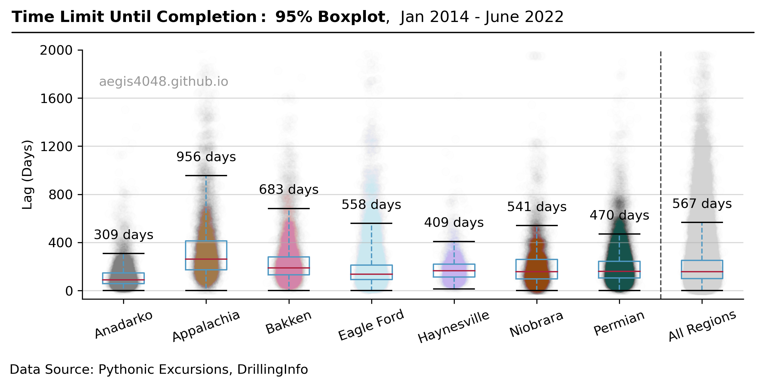
Figure 8: 95% Box plot of gap time between drilling and completion. The plot shows the time limit until completion for each basin. Each dot (very small, 99.5% transparency) represent one well of a basin. Upper whisker and the numeric annotation above it represent 95% upper limit. This means that wells with DUC time longer than the annotated number have less then 95% chance of ever being completed. Box plot for "All Regions" represent weighted average of all basins.
Related Posts
Quantifying The Impact Of Completion Delay Since Drilled On Production
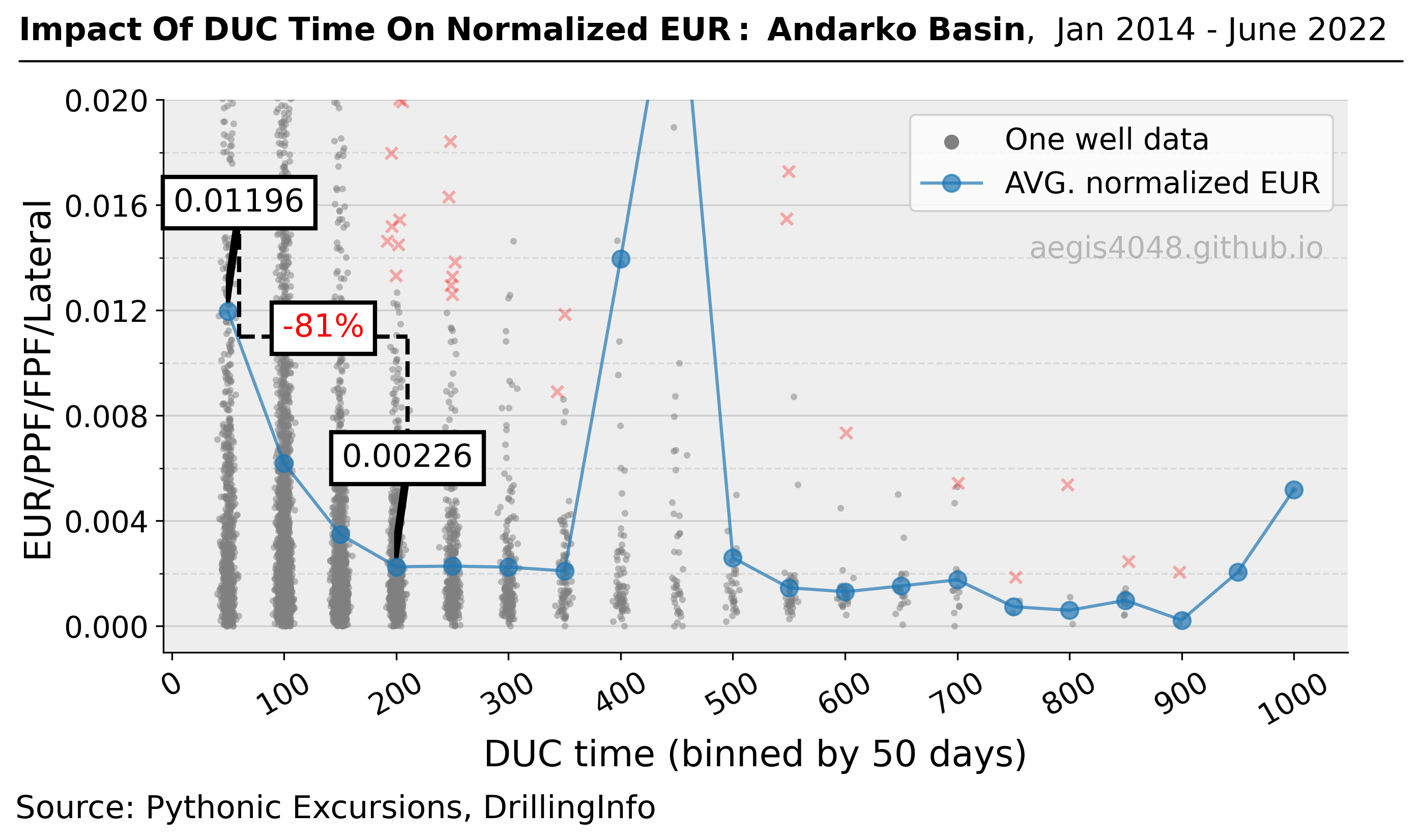
In times of unfavorable commodity prices, operators may delay completion after drilling in the hope of a price recovery. The study conducted in this article shows why this may not be a financially sound idea for certain basins by quantifying the impact of DUC time on normalized EURs.
H₂S Levels: Why High-Pressure Samples Don't Tell the Full Story
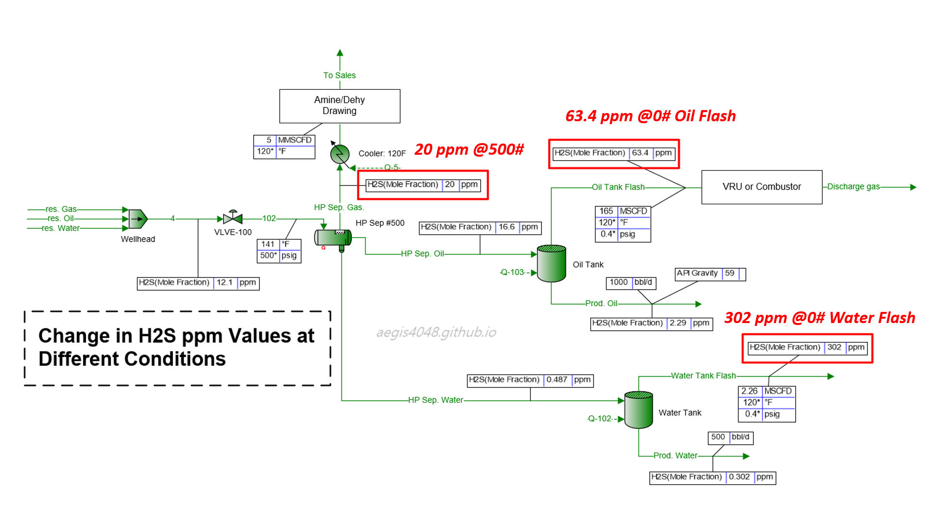
H₂S ppm levels obtained from high pressure applications (HP separators) are often re-used for low pressure applications (atmospheric tanks). H₂S levels soar 3~25 times at low pressures. This post explains the thermodynamics behind H2S ppm level variations and provide simulation results summary for practical applications.
Impact of Seasonal Changes on Storage Tank Emissions
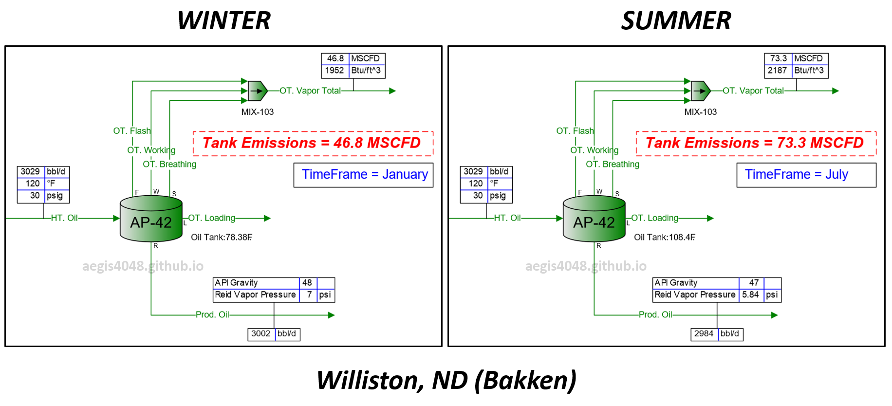
Storage tank temperatures rise in summer due to hot air, leading to higher emission volumes compared to winter. This temperature increase also impacts the dew point T, SG, and energy content (Btu/scf) of tank vapor. This post explains the phase behavior changes due to temperature shifts and provides a summary table with recommended operating capacity margins for emission handling systems across various regions.
Predicting VRU Economics/Downsizing Timing For Declining Wells
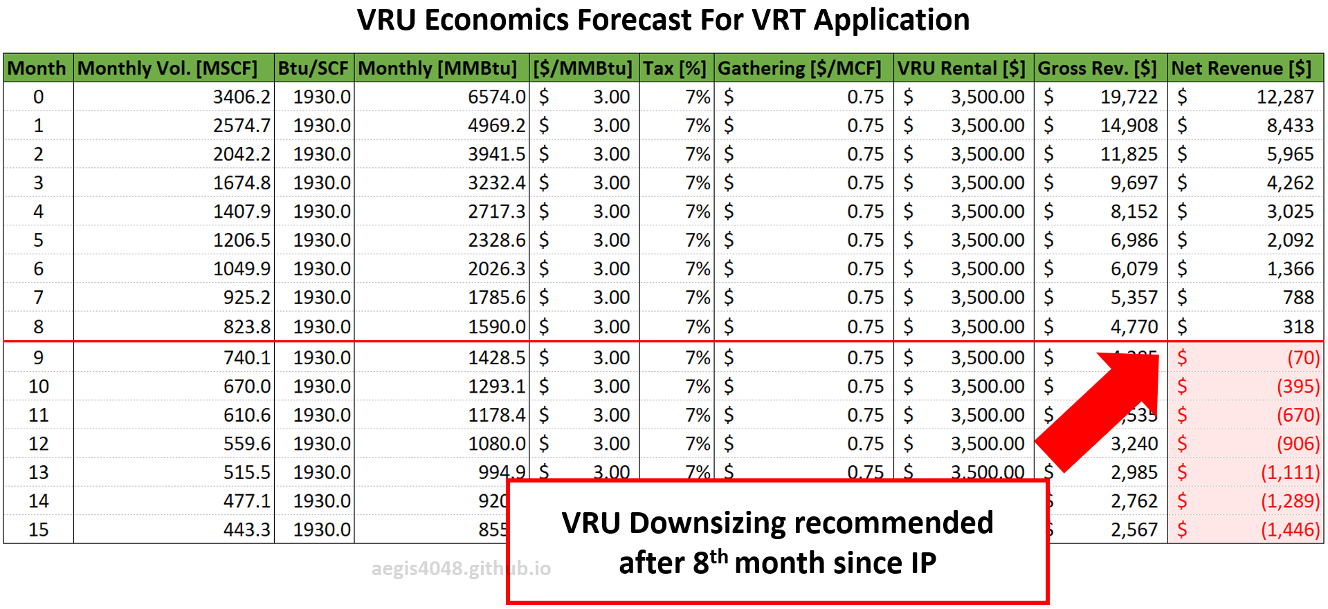
Flash gas rates from low-pressure vessels (heaters, VRTs, and tanks) can decline much faster than anticipated, mirroring the rate of oil decline. In some cases, they can drop by half within just 3 to 6 months from IP. This post presents monthly process simulation results that model the decline of flash gas from low-pressure vessels as the well declines. An Excel sheet is also provided to help calculate VRU economics.
Operation of Oil-Flooded Screw Compressor Explained
A detailed guide to oil-flooded screw compressor operations, covering compressor characteristics, operating capacity, unit P&ID, blowcase systems, control device mechanisms (valves and switches), pressure and temperature control, recycle mode, surface facility P&ID applications, lube oil contamination issues, electric vs. gas engine model comparisons, and more.