Impact of Seasonal Changes on Storage Tank Emissions
Category > Oil and Gas
Nov 11, 2024Concerns over global warming have led to stricter regulations, pushing oil and gas operators to produce "green" oil. One of the primary sources of emissions in the industry is from crude oil storage tanks. When hydrocarbon liquids are transferred into storage tanks from upstream separators, the crude oil is not fully stabilized yet and still contains some dissolved volatile gases, which vaporize inside the tank. These vapors accumulate, increasing pressure within the tank, requiring a pressure relief system to prevent explosions. Such relief mechanism can be either vapor recovery systems with compressors to capture vapors and send them to pipelines for sales, which are more environmentally friendly, or venting to air.
Vapor generation within a tank is influenced by two main factors: 1) the pressure drop from the upstream separator to the storage tank, and 2) the tank’s operating temperature. This article focuses on the latter—how the operating temperature of the tank, impacted by seasonal changes, affects emission volumes.
Here’s a quick takeaway for skimmers: Emission volumes are 22% (Texas) to 56% (North Dakota) higher in summer than in winter due to increased air temperatures. The summer-winter discrepancy is more pronounced in colder regions because of the greater seasonal temperature difference. See Table 2 below for a simulation summary across various scenarios. Note that this result is specific to the site simulation setups detailed below and may need fine tuning for different facility setups. However, the concept should still be generally applicable for most upstream facilities.
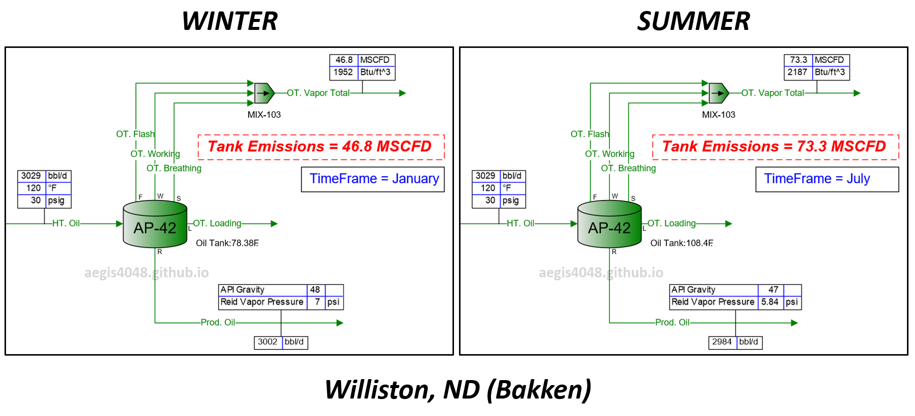
Figure 0: Flash volume simulation at atmospheric storage tanks using BR&E Promax. The setup assumes a liquid line from a heater operating at 30 psig and 120°F, dumping into an atmospheric tank at a rate of 3028 STBBL/D (34,600 lb/h) year-round. The plot shows increased emission rate at summer compared to winter due to increased ambient air temperature
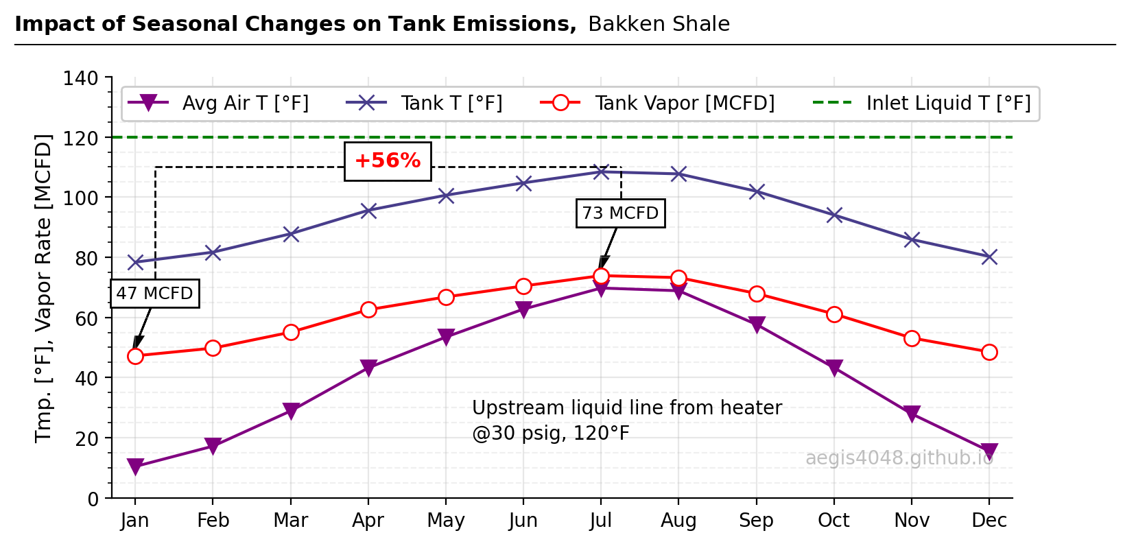
Figure 1: Flash volume simulation at atmospheric storage tanks using BR&E Promax. The setup assumes a liquid line from a heater operating at 30 psig and 120°F, dumping into an atmospheric tank at a rate of 3028 STBBL/D (34,600 lb/h) year-round. The red line represents vapor emission volumes from the tank. All conditions are held constant over 12 months, except for monthly ambient air temperature to isolate the effect of seasonal temperature on emissions. Williston, North Dakota, seasonal temperatures are used. Results show 47 MCFD emissions during winter and 73 MCFD during summer—a 56% increase. Elevated summer temperatures lead to higher emission volumes inside tanks. Refer to Figure 6 below for a process flow diagram of the site.
Source Code For Figure (1)
import pandas as pd
import numpy as np
import matplotlib.pyplot as plt
import matplotlib.ticker as ticker

df = pd.read_excel('https://aegis4048.github.io/downloads/notebooks/sample_data/seasonal_impact_data.xlsx', sheet_name='Sim Format 1')
df = df[df['Location'] == 'Williston, ND']

months = ['Jan', 'Feb', 'Mar', 'Apr', 'May', 'Jun', 'Jul', 'Aug', 'Sep', 'Oct', 'Nov', 'Dec']
x = np.array([i for i in range(12)])

fig, ax = plt.subplots(figsize=(8, 4))

ax.plot(x, df['AVG Air T (F)'], color='purple', label='Avg Air T [°F]', marker='v', markersize=8, linestyle='-')
ax.plot(x, df['Tank T (F)'], color='darkslateblue', label='Tank T [°F]', marker='x', markersize=8, linestyle='-')
ax.plot(x, df['Gas (MCFD)'], color='red', label='Tank Vapor [MCFD]', marker='o', markersize=8, linestyle='-', markerfacecolor='white')
ax.axhline(y=120, ls='--', color='green', label='Inlet Liquid T [°F]')


ax.set_ylim(0, 140)
ax.set_xlim(-0.3, 11.3)
ax.set_xticks(range(len(months)))
ax.set_xticklabels(months)

ax.yaxis.set_minor_locator(ticker.AutoMinorLocator())

ax.grid(axis='y', which='minor', linestyle='--', alpha=0.2)  # Minor grid lines
ax.grid(axis='both', which='major', linestyle='-', alpha=0.3)  # Major grid lines

ax.yaxis.get_major_ticks()[-1].gridline.set_visible(False)
ax.spines['right'].set_visible(False)
ax.spines.top.set_visible(False)


def annotate_arrows(data_y, num, tick_spacing, ymax, x_start=1, ox=0.2, fontsize=14, flip_y=False):
    '''
    data_y = y coordinate of the datapoint of interest
    num = index of the datapoint of interest
    tick_spacing = spacing between two major ticks
    ox = offset of x
    '''

    head_padding = ymax * 0.04                 # extra space between the datapoint of interest and arrowhead
    oy = ymax * 0.08                           # offset of y
    sx = x_start + (tick_spacing / 2) * num
    sy = data_y + head_padding

    if flip_y:
        oy = -ymax * 0.15
        sy = data_y - head_padding

    ax.arrow(sx + ox, sy + oy, -ox, -oy, head_width=0.1, head_length=ymax * 0.0333, fc='k', ec='k', lw=1)
    t1 = ax.text(sx + ox, sy + oy, str(int(data_y)) + ' MCFD', fontsize=fontsize, color='k', ha='center')
    t1.set_bbox(dict(facecolor='white', alpha=1, edgecolor='k', pad=3, lw=1))

    xytext = (sx + ox, sy + oy)

    return xytext

ymax = 160
fs=9
yloc=110
lw=1
spacing = abs(ax.get_xticks()[1] - ax.get_xticks()[2])

y1 = df['Gas (MCFD)'].values[0]
y2 = df['Gas (MCFD)'].values[6]

_1 = -2
_2 = 10

textxy1 = annotate_arrows(y1, _1 + 0.1, spacing, ymax, fontsize=fs)
textxy2 = annotate_arrows(y2, _2 + 0.1, spacing, ymax, fontsize=fs)

ax.plot([textxy1[0], textxy1[0]], [textxy1[1], yloc], lw=lw, color='k', ls='--')
ax.plot([textxy2[0], textxy2[0]], [textxy2[1], yloc], lw=lw, color='k', ls='--')
ax.plot([textxy1[0], textxy2[0]], [yloc, yloc], lw=lw, color='k', ls='--')

diff_percentage = '+' + str(int((y2 - y1)/y1 * 100)) + '%'
t1 = ax.text((textxy1[0] + textxy2[0])/2, yloc, diff_percentage, fontsize=11, color='red', ha='center', fontweight='bold')
t1.set_bbox(dict(facecolor='white', alpha=1, edgecolor='k', pad=5, lw=lw))

ax.legend(fontsize=10, ncol=4, loc='upper left', framealpha=1)

ax.set_ylabel('Tmp. [°F], Vapor Rate [MCFD]', fontsize=11)


ax.text(0.4, 0.2, 'Upstream liquid line from heater', fontsize=10, ha='left', transform=ax.transAxes, color='k')
ax.text(0.4, 0.14, '@30 psig, 120°F', fontsize=10, ha='left', transform=ax.transAxes, color='k')
ax.text(0.98, 0.08, 'aegis4048.github.io', fontsize=10, ha='right', transform=ax.transAxes, color='grey', alpha=0.5)
def setbold(txt):
    return ' '.join([r"$\bf{" + item + "}$" for item in txt.split(' ')])


bold_txt = setbold('Impact of Seasonal Changes on Tank Emissions, ')
plain_txt = 'Bakken Shale'
fig.suptitle(bold_txt + plain_txt, verticalalignment='top', x=0, horizontalalignment='left', fontsize=11)
yloc = 0.9
ax.annotate('', xy=(0.01, yloc + 0.01), xycoords='figure fraction', xytext=(1.02, yloc + 0.01),
            arrowprops=dict(arrowstyle="-", color='k', lw=0.7))

fig.tight_layout()
Contents
- 0. Introduction
- 1. Theories: Impact of temperature changes at separator vessels
- 1.1. Flash volume increase
- 1.2. Heavier separated gas
- 1.3. Higher energy content
- 1.4. Higher dew point temperature
- 1.5. More stabilized crude oil (RVP)
- 2. Simulation Setups
- 2.1. Site (operational) setups
- 2.2. Software (Promax) & calculation methods (AP42 Chap 7)
- 2.3. Regional ambient air temperatures data
- 3. Simulation results
- 4. Conclusion
1. Theories: Impact of temperature changes at separator vessels
Altering the operating temperature of a separator vessel impacts the phase behavior of fluids within it. This section provides a theoretical explanation of the effects of increasing temperature from low to high.

Figure 2: Simulation of flash behavior at low (100°F) vs high (150°F) temperatures, modeled with BR&E Promax. At higher operating temperatures in a separator vessel, the separated gas volume increases, with higher specific gravity, greater energy content (Btu/scf), and the separated crude becomes more stable, as indicated by a lower Reid Vapor Pressure value.
1.1. Flash volume increase
Increasing the operating temperature of a separator vessel (or storage tanks) raises the fluid mole fraction that escapes into the gas line. This phenomenon can be explained by phase envelopes, which show phase behavior changes under different pressures and temperatures.
Assume Figure 3 represents a phase envelope of a sample obtained from the liquid line of a separator operating at 200 psig. The blue circle on the figure sits on the 100% liquid bubble point curve, showing that by definition, the liquid is at its bubble point when it leaves any separator. This 200 psig liquid then flows into a heater operating at 50 psig and 120°F, causing the operating condition of the fluid to shift, represented by the red dashed circle. Flash gas is generated from the pressure drop from 200 psig to 50 psig, where 50% of the inlet liquid vaporizes and separates into the gas line of a heater.
Now assume the operator increases the heater temperature from 120°F to 150°F. The operating condition of the fluid in the heater shifts horizontally, and now sits on the 5% liquid (95% vapor) curve, shown by the solid red circle. The vapor fraction rises from 50% to 95% due to the temperature increase.
This demonstrates why raising temperature leads to higher flash volumes in any vessel, as the fluid’s operating condition moves closer to the 100% vapor dew point curve, increasing the vapor mole fraction. The same phase behavior applies to atmospheric tanks. When tank temperatures rise in summer due to hotter ambient air, more vapors are generated, as the fluid’s operating condition moves toward a higher vapor fraction curve.
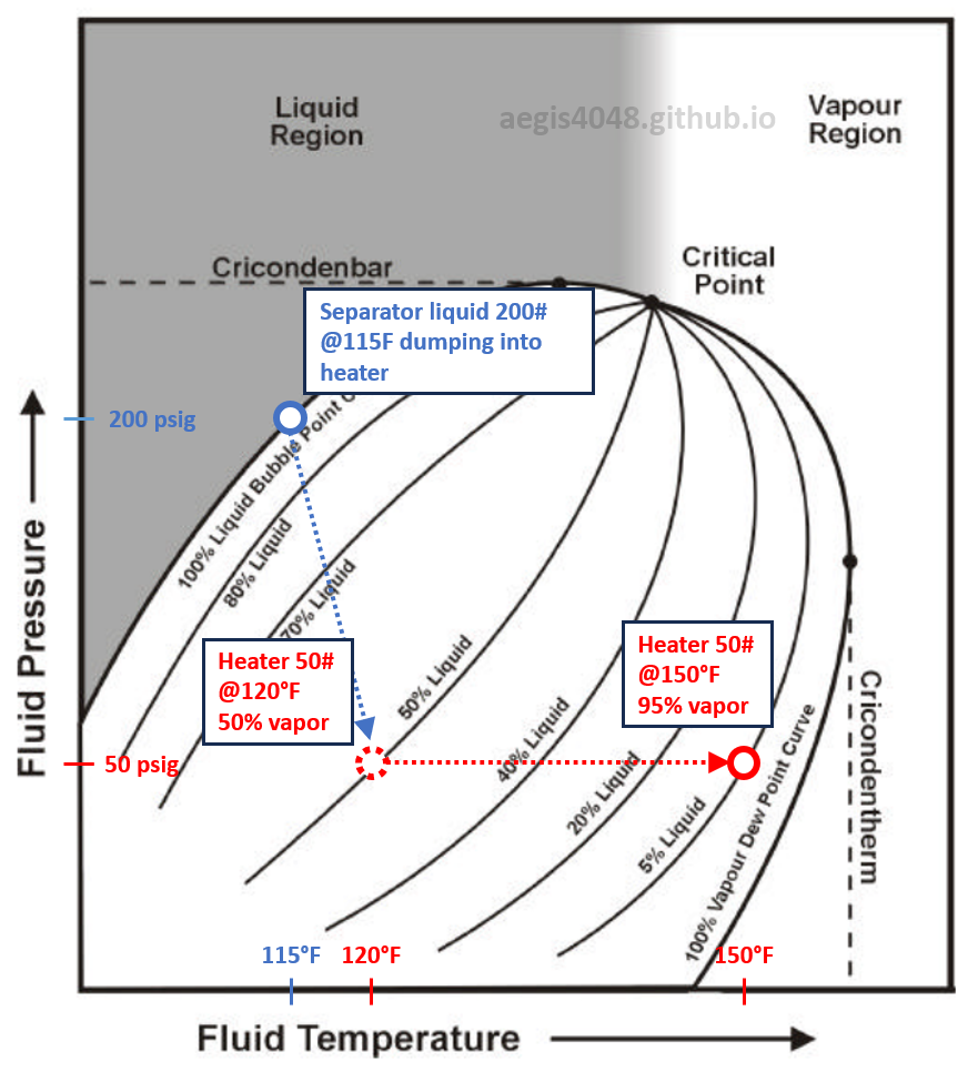
Figure 3: "Fake" phase envelope of a sample from the outlet liquid line of a separator operating at 200 psig, 115°F. This envelope is an educational illustration and is not derived from an actual sample. The original condition of the sample is marked by the blue circle. The liquid from the 200# separator flows into a heater operating at 50#, 120°F, represented by the dashed red circle. When the heater temperature is raised from 120°F to 150°F, the condition shifts horizontally toward the 100% vapor dew point curve. The envelope shows the varying vapor fractions of the fluid inside the heater at different operating conditions.
1.2. Heavier separated gas
Heavier hydrocarbon molecules vaporize more readily at elevated temperatures than at low temperatures, increasing the mole fraction of heavy-ends in the gas line and, consequently, the overall gas gravity. In Figure 2, the gas specific gravity (SG) rose from 0.816 to 0.956, and molecular weight (MW) from 23.6 to 27.7 lb/lbmol after a 50°F increase in vessel temperature.
1.3. Higher energy content
Heavier hydrocarbon molecules have higher energy content (Btu/scf). In Figure 2, gas energy content increased from 1396 Btu/scf to 1567 Btu/scf after a 50°F increase in vessel temperature.
Light-ends like methane have a MW of 16.04 lb/lbmol and an energy content of 1010 Btu/scf, whereas heavier-ends like n-pentane have an MW and energy content of 72.15 lb/lbmol and 4008.7 Btu/scf. In fact, gas molecular weight and energy content exhibit a nearly perfect linear correlation for paraffinic hydrocarbons (e.g., methane, ethane, butane, pentane, hexane), as shown in Figure 4.
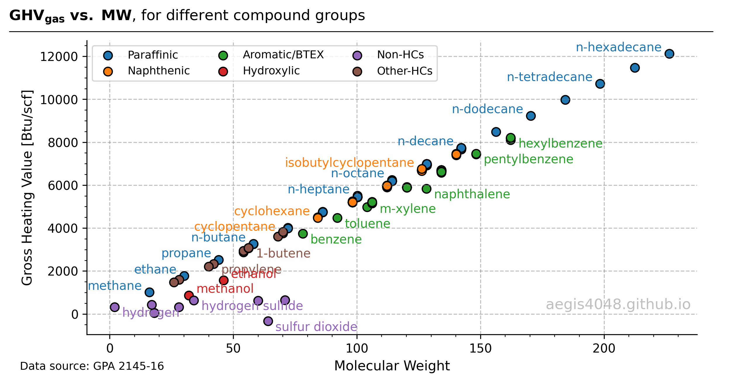
Figure 4: Scatter plot of known compounds upto n-hexadecane (C16H34) listed in the GPA 2145 table.
Source Code For Figure (4)
import pandas as pd
import matplotlib.pyplot as plt

df = pd.read_csv('https://aegis4048.github.io/downloads/notebooks/sample_data/GPA 2145-16_Compound_Properties_Table_English_Truncated_and_PNA_Identified.csv')

# Labeling for displaying texts
labels = ['methane', 'propane', 'n-butane', 'n-heptane', 'n-octane', 'n-decane', 'cyclohexane', 'cyclopentane', 'ethane',
'n-dodecane','n-tetradecane','n-hexadecane', 'methanol', 'ethanol', 'naphthalene', 'isobutylcyclopentane', 'hydrogen',
 'sulfur dioxide', 'hydrogen sulfide', 'toluene', 'benzene', 'm-xylene', 'pentylbenzene', 'hexylbenzene',
         'propylene', '1-butene'
         ]
df['Display Text'] = df['Compound'].isin(labels)

BTEX_idx = df[df['Is BTEX'] == True].index
aromatic_idx = df[df['Is Aromatic'] == True].index
non_HC_idx = df[df['Is Hydrocarbon'] == False].index
hydroxyl_idx = df[df['Is Hydroxyl'] == True].index
paraffinic_idx = df[df['Is Paraffinic'] == True].index
naphethenic_idx = df[df['Is Naphthenic'] == True].index
other_idx = df[df['Others'] == True].index
whole_idx = list(df.index)

x = df['Molar Mass [g/mol]']
y = df['Gross Heating Value Ideal Gas [Btu/ft^3]']

##################################### Plotting #######################################

fig, ax = plt.subplots(figsize=(8, 4.5))

alpha = 1
_1 = ax.scatter(x.loc[paraffinic_idx], y.loc[paraffinic_idx], s=50, edgecolor='k', alpha=alpha, label='Paraffinic')
_2 = ax.scatter(x.loc[naphethenic_idx], y.loc[naphethenic_idx], s=50, edgecolor='k', alpha=alpha, label='Naphthenic')
_3 = ax.scatter(x.loc[aromatic_idx], y.loc[aromatic_idx], s=50, edgecolor='k', alpha=alpha, label='Aromatic/BTEX')
_4 = ax.scatter(x.loc[hydroxyl_idx], y.loc[hydroxyl_idx], s=50, edgecolor='k', alpha=alpha, label='Hydroxylic')
_5 = ax.scatter(x.loc[non_HC_idx], y.loc[non_HC_idx], s=50, edgecolor='k', alpha=alpha, label='Non-HCs')
_6 = ax.scatter(x.loc[other_idx], y.loc[other_idx], s=50, edgecolor='k', alpha=alpha, label='Other-HCs')

c1 = _1.get_facecolor()[0]
c2 = _2.get_facecolor()[0]
c3 = _3.get_facecolor()[0]
c4 = _4.get_facecolor()[0]
c5 = _5.get_facecolor()[0]
c6 = _6.get_facecolor()[0]

ax.legend(fontsize=9, ncol=3)

texts = df['Compound']
for i, txt in enumerate(texts):
    if df['Display Text'].loc[i]:
        c = c5
        ha ='left'
        va = 'top'

        if df['Is Paraffinic'].loc[i]:
            c = c1
            ha ='right'
            va = 'bottom'
        if df['Is Naphthenic'].loc[i]:
            c = c2
            ha ='right'
            va = 'bottom'
        if df['Is Aromatic'].loc[i]:
            c = c3
            va = 'top'
            ha = 'left'
        if df['Is Hydroxyl'].loc[i]:
            c = c4
            va = 'bottom'
            ha = 'left'
        if df['Others'].loc[i]:
            c = c6
            va = 'top'
            ha = 'left'

        if ha == 'left':
            icr = 3
        else:
            icr= -3

        ax.annotate(txt, (x.loc[i] + icr, y.iloc[i]), fontsize=10, c=c, ha=ha, va=va)

ax.minorticks_on()
ax.grid(axis='y', which='major', linestyle='--', color='grey', alpha=0.5)
#ax.grid(axis='y', which='minor', linestyle='--', color='grey', alpha=0.2)
#ax.grid(axis='x', which='minor', color='grey', linestyle='--', alpha=0.2)
ax.grid(axis='x', which='major', color='grey', linestyle='--', alpha=0.5)
ax.spines['top'].set_visible(False)
ax.spines['right'].set_visible(False)

ax.set_xlabel('Molecular Weight', fontsize=11)
ax.set_ylabel('Gross Heating Value [Btu/scf]', fontsize=11)
ax.text(0.99, 0.1, 'aegis4048.github.io', fontsize=12, ha='right', va='center',
    transform=ax.transAxes, color='grey', alpha=0.5)

#ax.set_xlim(0, 1)
#ax.set_ylim(10000, 30000)

def setbold(txt):
    return ' '.join([r"$\bf{" + item + "}$" for item in txt.split(' ')])

bold_txt = setbold('GHV_{gas} vs. MW')
plain_txt = ', for different compound groups'

fig.suptitle(bold_txt + plain_txt, verticalalignment='top', x=0, horizontalalignment='left', fontsize=12, y=0.96)
yloc = 0.88
ax.annotate('', xy=(0.01, yloc + 0.01), xycoords='figure fraction', xytext=(1.02, yloc + 0.01),
            arrowprops=dict(arrowstyle="-", color='k', lw=0.7))

ax.annotate('Data source: GPA 2145-16', xy=(-0.11, -.12), xycoords='axes fraction', fontsize=9)

fig.tight_layout()
1.4. Higher dew point temperature
Gas dew point temperatures are critical for compressor applications. In high-pressure setups, like those using reciprocating compressors, accurate dew point calculations help define design parameters for compression chambers and ensure liquid knockout scrubbers are properly sized. For lower-pressure applications (below 300 psig), such as oil-flooded screw compressors, dew point control is essential to prevent liquid condensation during compression, which can lead to lube oil contamination.
The specific gravity of a mixture affects its dew and bubble points. While the relationship isn’t perfectly linear, heavier mixtures generally exhibit higher dew points at the same pressure than lighter ones. Figure 5 illustrates this effect with vapor samples from the same tank in different seasons. The summer sample, with a higher specific gravity, has a dew point temperature of 222°F at 600 psig, while the lighter winter sample has a dew point of 184°F—a significant difference that could impact operations.
In this 600 psig scenario, which exceeds the operating capacity of screw compressors, reciprocating compressors are required. For reciprocating compressors, scrubber sizing for liquid knockout is heavily influenced by dew point temperature. A scrubber sized based on a winter sample may be undersized for summer operations, risking liquid carryover during higher-temperature seasons.
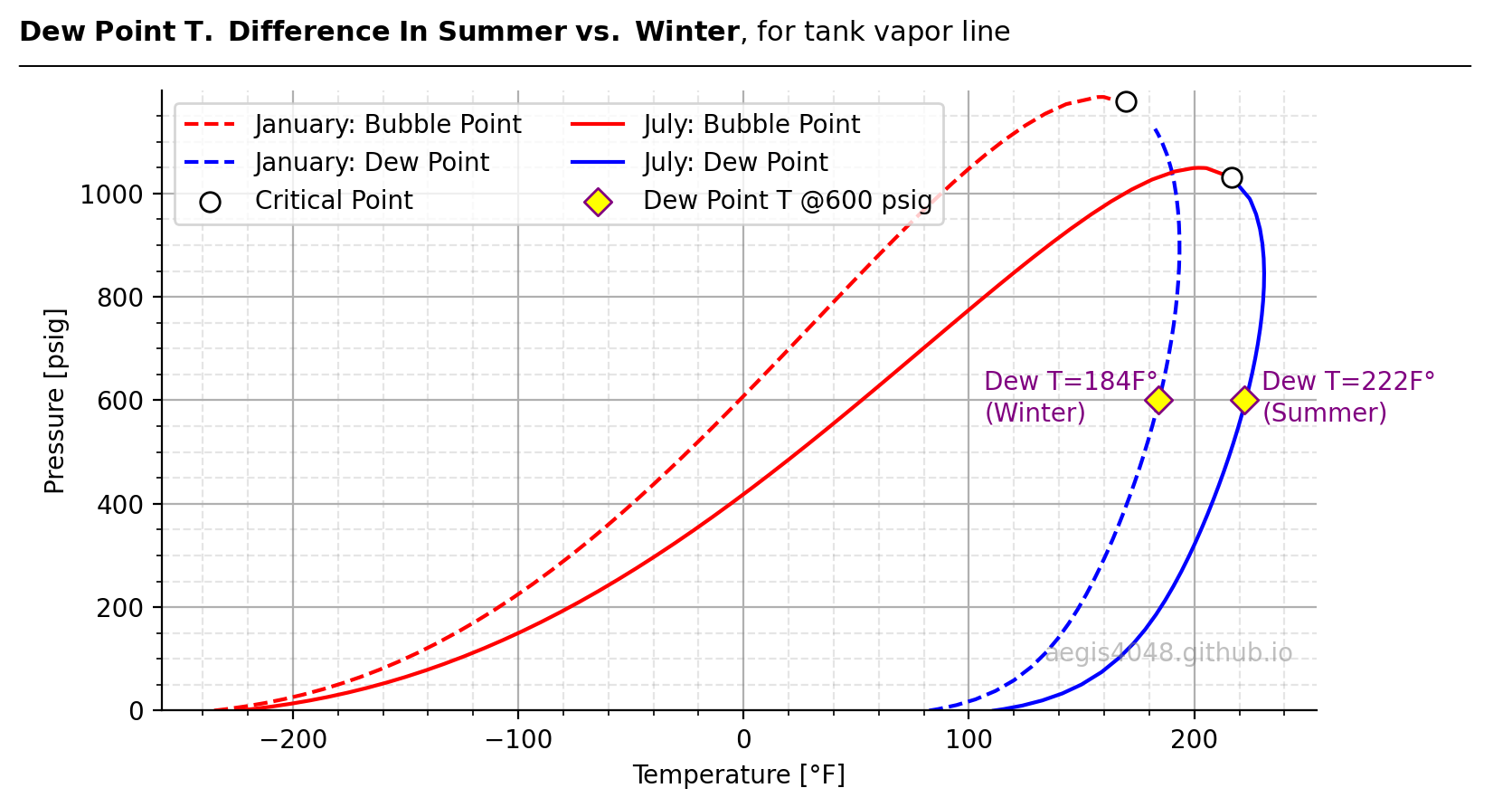
Figure 5: Phase envelopes of tank vapor samples under summer and winter conditions. The dashed line represents the winter sample, while the solid line represents the summer sample. The winter sample has an energy content of 2021 Btu/scf, whereas the summer sample is richer at 2317 Btu/scf. Yellow diamonds mark the dew point temperatures at 600 psig, showing the summer sample's higher dew point of 222°F compared to the winter sample’s 184°F.
Source Code For Figure (5)
import pandas as pd
import numpy as np
import matplotlib.pyplot as plt

df = pd.read_excel('https://aegis4048.github.io/downloads/notebooks/sample_data/seasonal_impact_data.xlsx', sheet_name='Bakken Envelope')
df.sort_values(by='Month')

fig, ax = plt.subplots(figsize=(8, 4.5))

months = sorted(list(set(df['Month'])))
lss = ['--', '-']
for ls, month in zip(lss, months):

    df_cur = df[df['Month'] == month]
    x_crit = df_cur['Critical T [°F]'].values[0]
    y_crit = df_cur['Critical P [psig]'].values[0]
    df_cur = df_cur[df_cur['Pressure [psig]'] - y_crit < 20] # filter to remove outliers in sim results


    x_dew = df_cur[df_cur['Curve Type'] == 'Dew']['Temperature [°F]'].values
    y_dew = df_cur[df_cur['Curve Type'] == 'Dew']['Pressure [psig]'].values

    x_bubble = df_cur[df_cur['Curve Type'] == 'Bubble']['Temperature [°F]'].values
    y_bubble = df_cur[df_cur['Curve Type'] == 'Bubble']['Pressure [psig]'].values

    ax.plot(x_bubble, y_bubble, label=month + ': Bubble Point', ls=ls, color='red')
    ax.plot(x_dew, y_dew, label=month + ': Dew Point', ls=ls, color='blue')
    ax.scatter(x_crit, y_crit, s=60, edgecolor='k', fc='white', zorder=3, label='Critical Point')


ax.set_ylim(0, 1199)
ax.set_xlabel('Temperature [°F]')
ax.set_ylabel('Pressure [psig]')


ax.grid(True)
ax.spines['top'].set_visible(False)
ax.spines['right'].set_visible(False)

ax.minorticks_on()
ax.grid(axis='both', which='minor', color='grey', linestyle='--', alpha=0.2)

ax.scatter(184, 600, marker='D', s=60, fc='yellow', edgecolor='purple', zorder=10, label='Dew Point T @600 psig')
ax.scatter(222, 600, marker='D', s=60, fc='yellow', edgecolor='purple', zorder=10)

ax.text(184, 610, 'Dew T=184F°', fontsize=10, ha='right', va='bottom', color='purple')
ax.text(107, 550, '(Winter)', fontsize=10, ha='left', va='bottom', color='purple')

ax.text(230, 610, 'Dew T=222F°', fontsize=10, ha='left', va='bottom', color='purple')
ax.text(230, 550, '(Summer)', fontsize=10, ha='left', va='bottom', color='purple')

handles, labels = ax.get_legend_handles_labels()
handles.pop(-2)
labels.pop(-2)
ax.legend(handles[:], labels[:], ncol=2)


ax.text(0.98, 0.08, 'aegis4048.github.io', fontsize=10, ha='right', transform=ax.transAxes, color='grey', alpha=0.5)
def setbold(txt):
    return ' '.join([r"$\bf{" + item + "}$" for item in txt.split(' ')])

bold_txt = setbold('Dew Point T. Difference In Summer vs. Winter')
plain_txt = ', for tank vapor line'
fig.suptitle(bold_txt + plain_txt, verticalalignment='top', x=0, horizontalalignment='left', fontsize=11)
yloc = 0.9
ax.annotate('', xy=(0.01, yloc + 0.01), xycoords='figure fraction', xytext=(1.02, yloc + 0.01),
            arrowprops=dict(arrowstyle="-", color='k', lw=0.7))


fig.tight_layout()
1.5. More stabilized crude oil (RVP)
Increased vapor generation rate inside a tank means that the stored liquid becomes more stabilized, with less volatiles because those dissolved volatiles in the crude escaped the system through a vent line (vented to air, captured, or flared). This can be seen in Figure 2, in which the Reid Vapor Pressure (RVP) for higher temperature vessel (150F) is lower (RVP=8.84 psi) than the lower T vessel (100F, RVP=9.74 psi). Lower RVP means more stable crude. EPA Gasoline Reid Vapor Pressure requires storage gasoline to have RVP value lower than 9 to 7.8 psi to reduce emissions of volatile organic compounds (VOCs).
2. Simulation Setups
This section details the simulation setups and assumptions used to investigate the impact of seasonal temperature changes on storage tank emissions.
2.1. Site (operational) setups
A generic upstream facility structure is used for simulations. Reservoir fluid flows up the production tubing to the wellhead, then to a 2-phase separator, a heater treater, and finally to atmospheric storage tanks. Figure 6 shows facility modeling done with Promax.
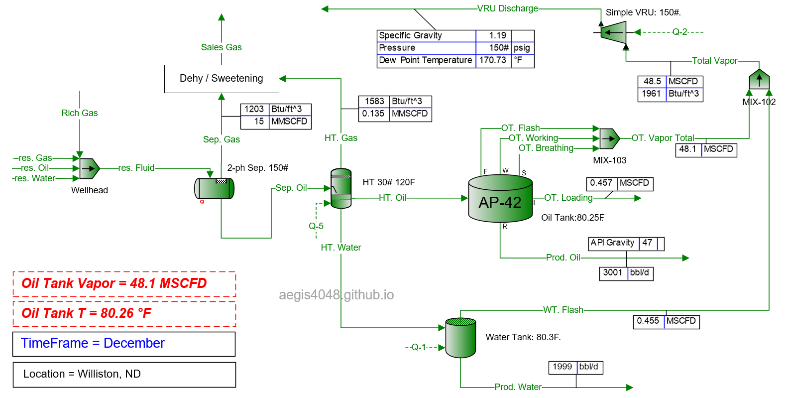
Figure 6: Generic upstream facility modeling done in BR&E Promax. This simulation assumes an ambient air temperature of 15.5°F in Williston, ND, in December (see Table 1 below for regional seasonal temperature data). All operating parameters are held constant except timeframe (month) and ambient air temperature across various locations to observe the impact of seasonal temperature changes on tank emission volumes.
Assumptions
- Generic upstream oil and gas facility with wellhead.
- 2-phase separator operating at 150 psig.
- VRU discharge pressure set equal to separator pressure: 150 psig.
- Wellhead temperature: 140°F.
- 3-phase heater treater operating at 30 psig, 120°F.
- Atmospheric oil tank operating at 0.6 psig, with temperature affected by ambient air and incoming fluid temperature.
- 47° API oil.
- Sales gas energy content: 1203 Btu/scf, specific gravity: 0.69.
- Facility production rates: 15 MMSCFD (gas), 3000 BOPD (oil), and 2000 BWPD (water).
- Four standard 750 BBL API 12F oil storage tanks (15.5' x 24', tan-colored).
- Water tank sizing omitted for simplicity; water tank temperature assumed to match oil tank temperature.
- Timeframe (month) and location are the only variables that change for each simulation run.
- Compression boost for heater treater gas to salesline is omitted for simplicity, as it doesn't affect downstream tank conditions. Common handling strategies for HT gas include: 1) Installing an additional booster compressor dedicated to HT gas, 2) Routing the gas line to tank inlets so HT gas can be handled by the tank VRU along with tank vapors, and 3) Using a 3-way control system to enable a single compressor to handle both the tank gas line (0.6 psig) and HT gas line (30 psig).
Notes: Flash, Breathing, Working, and Loading Losses
AP-42 calculation methods (see below) for atmospheric storage tanks provide calculation methods for four vaporization types: flash, working, breathing, and loading.
Flash: Rapid release of dissolved gases from liquid due to a pressure drop from high to low pressure
Working: Occurs during tank filling operations. As the liquid level rises, vapor space pressure increases, expelling vapors through the roof vent. Although not included in AP-42 methods, working loss can also involve vaporization from turbulence and vapor/liquid contact due to splash loading. Downcomers (submerged loading) help reduce splash losses.
Breathing: Vaporization caused by day (hot) vs night (cold) temperature differences.
Loading: Results from inefficiencies during truck-loading operations.
2.2. Software (Promax) & calculation methods (AP42 Chap 7)
BR&E Promax is a process simulation software widely used in the oil and gas industry. One of it's features include implementation storage tank emission calculation methods outlined in AP42 Chapter 7: Liquid Storage Tanks. The chapter explains emission mechanism for fixed and floating roof tanks for various tank dimensions, structures, paint color, location, month of year, etc. The site simulation setup for this article assumes upstream facility, which traditionally use standardized API 12F tanks. Some of the key inputs used in AP42 can be taken from standard API 12F tank specs such as dimensions (15.5' x 24' for 750 BBL capacity), design pressure (16 oz vent and 1 oz vacuum safety), and tank geometry (fixed roof vertical cylinder).
Notes: API 12F Tanks
API 12F tanks are standardized storage tanks primarily used in upstream oil and gas production facilities to store crude oil and produced water at atmospheric pressure. Designed and built to the specifications set by the American Petroleum Institute (API), these tanks are widely used due to their reliability, uniformity, and compatibility with industry standards.
Standardized Design: API 12F tanks follow strict specifications for dimensions, shape, thickness, reinforcement details, and materials (typically carbon steel) with welded construction to ensure durability and strength. Standardized capacities range from 90 to 1,000 BBL.
Design Pressure: Tanks are equipped with a pressure relief mechanism to keep operating pressure below 16 oz (1 psig) to prevent explosion, and a vacuum relief mechanism to stay above 1 oz, preventing implosion.
Compliance and Safety: For facilities near commercial or residential areas, API guidelines recommend an additional pressure/vacuum relief mechanism for emergency scenarios, set to release at 24 oz for overpressure and 1.5 oz for vacuum. Most remote wellsites in the field do not require this extra installation.
Vent Line Connection Sizing: The guidelines specify minimum pipe diameters for roof vent lines, especially critical when not venting directly to air. This sizing ensures minimal pressure drop between the vent line and emission control system (e.g., VRU or flare). Typical tank operating pressure is below 0.6 psig, allowing only a small margin to ensure vapor flow to the VRU or flare. Even minor pressure drops from friction can restrict flow, leading to overpressurization and triggering relief valves on the tanks, which results in unwanted emissions. Pipe diameters must be large enough to prevent any pressure drop due to friction that could block flow.
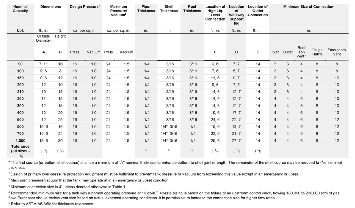
Figure A: API 12F tank standard specifications at different nominal capacities, screenshot from API 12F 13th edition, 2019.
2.3. Regional ambient air temperatures data
AP-42 Chapter 7 Table 7.1-7. Meteorological Data for Selected U.S. Locations provides average monthly temperatures for all 12 months across various locations. Key oil and gas regions' average temperatures are summarized in Table 1. Notably, the Bakken region shows the largest seasonal temperature difference between summer and winter, leading to the highest seasonal variation in emission volumes (56%), compared to regions like Eagle Ford (22%), as summarized in Table 2.

Table 1: Seasonal temperature data for key U.S. locations, selected from AP-42 Chapter 7 Table 7.1-7, matched to corresponding basins. Rows are sorted by locations with the highest to lowest temperature differences between January and July.
3. Simulation results
Table 2 shows storage tank simulation results for quantifying the seasonal contrast for summer vs winter for tank vapor rates and other properties. The colder the region, such as in Bakken, Powder River, and Marcellus, the greater was the differences due to greater seosonal T difference than warmer regions in Texas. Bakken region showed the greated seasonal tank flash rate increase of 56% in summer compared to winter, while Eagleford showed the lowest increase of 22%.
My simulation result table can be downloaded from here: Storage Tank Emissions Simulation Data (seasonal_impact_data.xlsx)
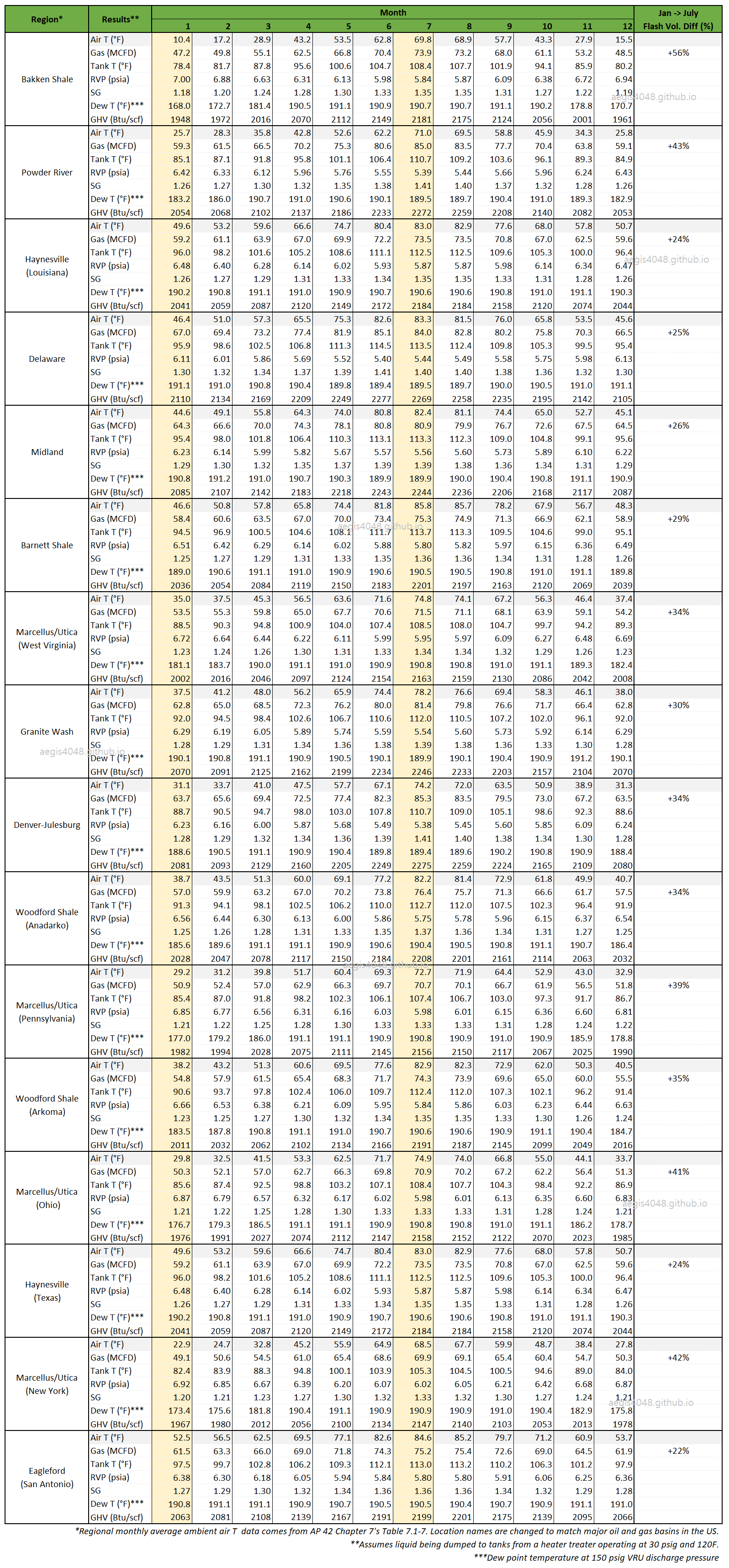
Table 2: Storage tank simulation result table contrasting seasonal differences for summer vs. winter for tank vapor line with assumed setups detailed in Simulation Setups above. Air T (°F) is regional seasonal ambient air temperature taken from Table 1. Tank T (°F) is the operating temperature of the storage tank, affected by upstream heater treater temperature (120F in this setup), and ambient air temperature. RVP (psia), Reid Vapor Pressure, is taken from "Prod. Oil" stream in Figure 6. Dew T (°F) taken from "VRU Discharge" stream in Figure 6. This is the dew point temperature of the compressed gas at 150 psig. The rest of the properties, Gas (MCFD), SG, and GHV (Btu/scf) are taken from stream "Total Vapor". The biggest seasonal contrast occur between Jan vs. July due to the greatest air T difference.
4. Conclusion
1. When an upstream liquid line flows into a separator vessel, it enters as 100% liquid, with separation occurring inside the vessel. Changing the vessel’s operating temperature or pressure shifts the fluid’s position on a phase envelope, altering its vapor fraction inside a vessel (see 1.1. Flash volume increase and Figure 3 above), and compositions of the separated outlet lines. This same phenomenon applies to atmospheric applications like storage tanks.
2. Increasing a vessel’s temperature raises flash volume, producing a heavier (richer) separated gas with higher energy content and a higher dew point temperature at a given pressure. For the oil line, higher temperature lowers the crude oil’s Reid Vapor Pressure (RVP), meaning the crude is more stabilized as more volatiles have separated into the gas line.
3. Emission handling systems (flares or vapor recovery units) should be sized to manage increased gas volume and gravity during summer compared to winter.
4. Summer flash volume increases ranged from 20–30% in Texas regions (Eagle Ford, Delaware, Midland) and from 50–60% in North Dakota (Bakken), compared to winter.
5. Colder regions have larger temperature differences between summer and winter, resulting in a greater seasonal variation in tank vapor emissions.
6. See Table 2 for a summary of simulation results showing the impact of monthly air temperature on tank vapor emissions by region.
