Predicting VRU Economics/Downsizing Timing For Declining Wells
Category > Oil and Gas
Feb 25, 2025Many producers, when sizing vapor recovery units (VRUs) or signing long-term contracts for them, tend to overlook an important factor: the inevitable decline of flash gas rates over time. Flash gas rates at heater treaters (HT), vapor recovery towers (VRT), and tanks follow a similar decline pattern to well production, yet it's a common misconception that these rates will remain steady or only decrease marginally.
Working at a compressor company, I’ve seen firsthand how producers expect flash gas rates to hold relatively flat or marginally decline; the flash gas rates go down much quicker than they think. While the oil decline rate plays the largest role in this reduction, many still fail to account for it when planning for long-term operations. It's not necessarily that they don't know about the decline, but rather that they simply forget to think about it because VRUs are not their primary concern. Downsizing is often not done in a timely manner because it’s overlooked, and as a result, VRUs quickly become oversized and uneconomical. It's also common to see a well experience more than a 50% drop in production within the first few months since initial production (IP), making this issue even more critical.
KEY DELIVERABLES OF THIS ARTICLE:
Notes: Clarifications on Terms
Low Pressure Vessels: Refers to vessels such as low-pressure separators, heater treaters (HT), vapor recovery towers (VRT), or tanks. These vessels are downstream of the primary separator and operate at pressures lower than the sales line pressure.
Sales (Produced) Gas: High-pressure gas from the primary separator that operates around the sales line pressure, typically lean gas with a BTU content of 1050-1600 Btu/scf.
Flash Gas: Gas volumes coming from low-pressure vessels operating below sales line pressure. These gases are richer, typically ranging from 1400-3000 Btu/scf, and lack sufficient pressure to enter the sales line. Flash gas can either be flared or recovered by VRUs that compress the gas to above sales line pressure. Flash gas is often distinguished from sales gas coming from the primary high pressure separator.
VRU Flowrate: For the purpose of this article, VRU flowrate is synonymous to flash gas.
VRU: Vapor Recovery Unit, VRU, is one application of a compressor. The compressor type can be rotary vane, rotary screw, or reciprocating.
1. Industry Practices for VRU Sizing
When a new facility is being built, engineers typically input the expected initial production (IP) flowrates into process simulation software to estimate the expected flash gas flowrates at low-pressure vessels. In the absence of process simulation software, many producers and vendors rely on ballpark estimates using flat scf/bbl numbers based on regional experience to predict flash gas volumes. While quick, this scf/bbl method doesn't account for the operating pressure of the vessels, leading to inaccuracies. These projected rates are then provided to VRU vendors, who size the equipment and provide quotes based on the high IP flowrates. Since these flowrates are often large, the VRU is sized to handle peak capacity, resulting in a costly investment. However, as the well declines, these high flowrates no longer match reality, and the oversized VRU quickly becomes uneconomical. Unfortunately, this issue is often realized too late, as VRUs are not always the primary concern for producers.
Some keen producers who pay attention to VRUs predict monthly VRU flowrate declines using process simulations or by applying an oil decline curve to the IP flash gas rates. For example, if oil is expected to drop by 50% in the first 4 months and the IP flash gas rate is initially calculated to be 100 MCFD, the flash gas rate will decrease to around 50 MCFD in 4 months. The large and expensive compressor sized for peak initial flowrate will either be downsized or moved to a different location with similar production capacity to ensure its continued economic viability.
2. Predicting flash gas flowrates with process simulations
The purpose of this section is to demonstrate that the declining flash gas rates at low-pressure vessels closely follow the oil decline curve and to highlight that gas decline has a minor impact compared to oil decline. BR&E Promax software is used for the simulations.
2.1. Site (operational) setups
A generic upstream facility structure is used for simulations. Reservoir fluid flows up the production tubing to the wellhead, then to the first-stage 2-phase separator, followed by a second-stage 2-phase separator operating 5 psi lower than the first stage, a heater treater, VRT, and finally to atmospheric storage tanks. The purpose of the second-stage separator is to separate the liquids entrained in the gas stream from the first-stage separator. Figure 1 shows the facility model created in Promax for IP flowrates. This model serves as the base, accepting monthly declining oil, gas, and water rates (Section 2.2) as inputs, and returning declining rates of downstream flash gases as outputs (Table 2).
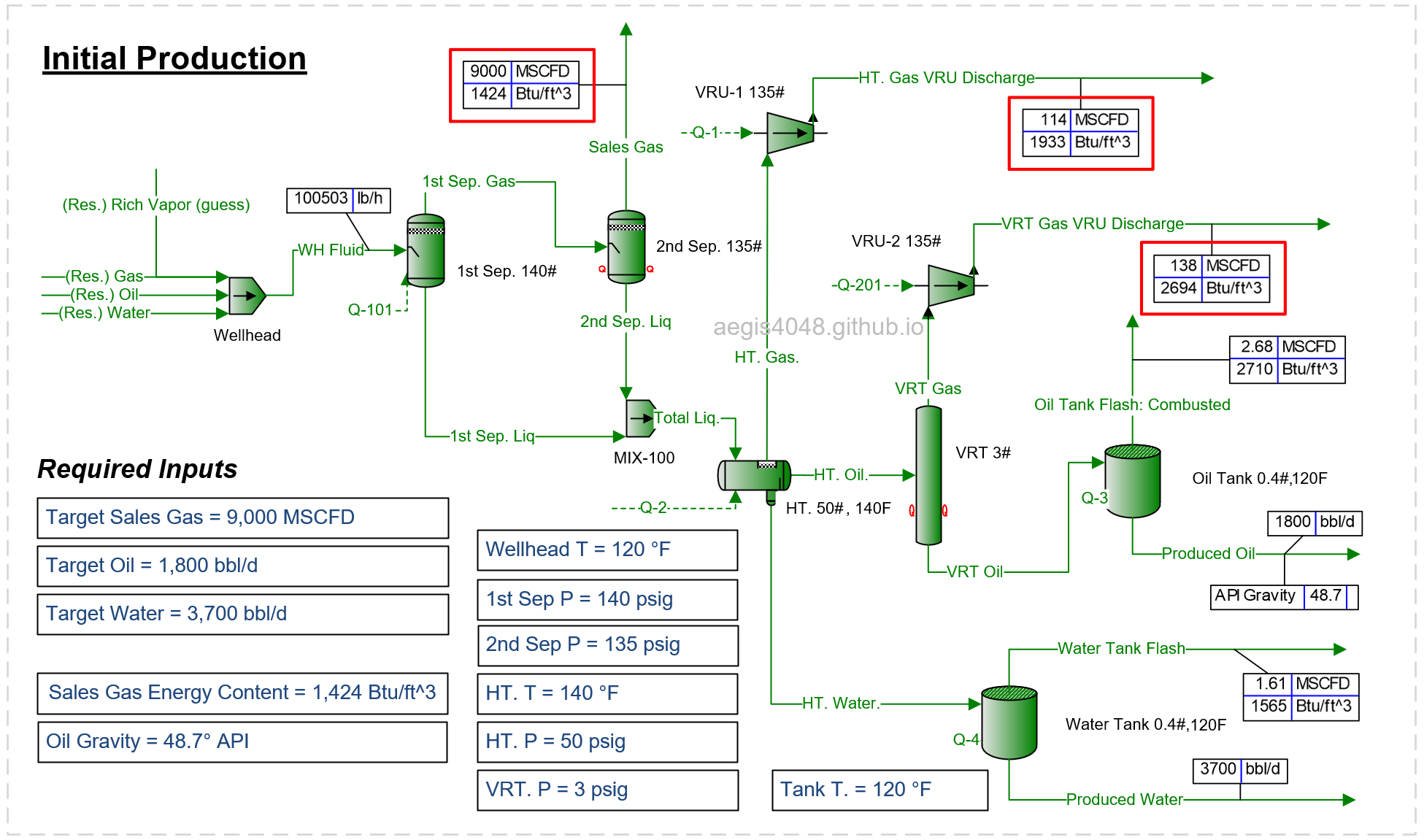
Figure 1: Generic upstream facility modeling done in BR&E Promax. IP rates of 9 MMSCFD (gas), 1800 BOPD (oil), and 3700 BWPD (water) are assumed. Numbers in the red boxes show produced and flash gas rates.
Assumptions
- Generic upstream oil and gas facility with wellhead.
- 2 stage 2-phase separators operating at 140 and 135 psig.
- VRU discharge pressure set equal to 2nd separator pressure: 135 psig.
- Details of VRU components (ex: cooler, knockout scrubbers) are omitted for simplicity.
- Wellhead temperature: 120°F.
- 3-phase heater treater operating at 50 psig, 140°F.
- Atmospheric oil tank operating at 0.4 psig, 120°F
- 48° API oil.
- Sales gas energy content: around 1420 Btu/scf
- Facility Initial production rates: 9 MMSCFD (gas), 1800 BOPD (oil), and 3700 BWPD (water).
- Future declining production rates are predicted by Figure 2
- BR&E Promax solver is used to solve for flowrates at wellhead. Solver adjusts inlet (wellhead) flowrates to match production rates at measurement points (sales gas meter/LACT/trucking/etc) leaving the system.
- Realistic oil and gas compositions used.
2.2. Simulation scenarios
To observe the impact of well decline on downstream flash gas flowrates, decline curve analysis (DCA) parameters are set up to simulate declining oil, gas, and water flowrates. Oil and water decline rates (with water having no impact on flash gas volumes) are fixed to isolate the impact of gas declines. Three scenarios are considered: 1) gas declining faster than oil, 2) gas declining slower than oil, and 3) gas declining at the same rate as oil. The DCA parameters shown in Figure 2 are used to create hypothetical declining well production rates, as shown in Figures 3, 4, and 5. These rates are then fed into the Promax model to predict flash gas rates at low-pressure vessels.
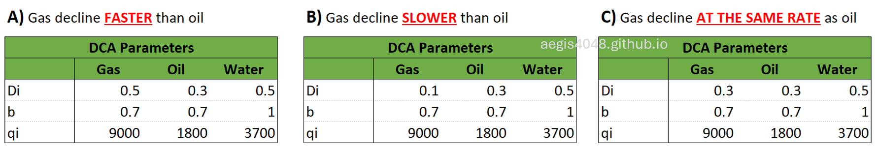
Figure 2: DCA parameters used to simulate declining well flowrates. Oil and water decline rates are fixed to observe the sole impact of produced gas decline on flash gas declines. Note that the b-factor is set the same for both oil and gas in all scenarios for ease of decline curve comparisons.
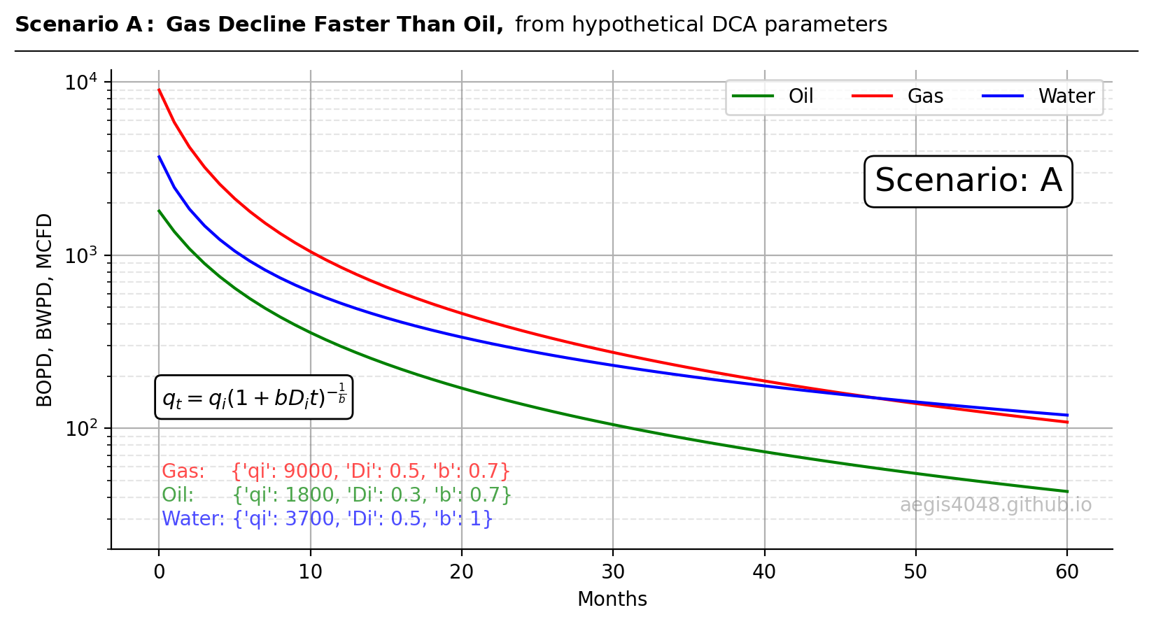
Figure 3: Well decline curve prediction from the DCA parameters in scenario A of Figure 2.
Source Code For Figure (3)
import pandas as pd
import numpy as np
import matplotlib.pyplot as plt


def general_decline(t, qi, Di, b):
    """
    Arps' decline equation for production decline modeling.

    Args:
        t (array-like): Time values.
        qi (float): Initial production rate.
        Di (float): Initial decline rate.
        b (float): Decline exponent.

    Returns:
        array-like: Production rate at time t.
    """
    return qi * (1 + b * Di * t) ** (-1 / b)

params = {
    'Oil': {'qi': 1800, 'Di': 0.3, 'b': .7},
    'Gas': {'qi': 9000, 'Di': 0.5, 'b': 0.7},
    'Water': {'qi': 3700, 'Di': 0.5, 'b': 1}
}

x = np.arange(0, 61)
fits = {
    'Oil': [],
    'Gas': [],
    'Water': [],
}
for key in params.keys():
    target_params = list(params[key].values())
    fits[key] = general_decline(x, *target_params)
df = pd.DataFrame.from_dict(fits)
df['Count'] = x

fig, ax = plt.subplots(figsize=(8, 4.5))

oc = 'green'
gc = 'red'
wc = 'blue'


ax.plot(df['Count'], df['Oil'], c=oc, label='Oil')
ax.plot(df['Count'], df['Gas'], c=gc, label='Gas')
ax.plot(df['Count'], df['Water'], c=wc, label='Water')


ax.set_xlabel('Months')
ax.set_ylabel('BOPD, BWPD, MCFD')


ax.grid(True)
ax.spines['top'].set_visible(False)
ax.spines['right'].set_visible(False)

#ax.minorticks_on()
ax.grid(axis='both', which='minor', color='grey', linestyle='--', alpha=0.2)
ax.legend(ncol=6, loc='upper right')

ymax = 10000
ymin = 10
xmax = ax.get_xlim()[1]
xmin = 0 - xmax * 0.05
ax.set_yscale('log')
ax.set_ylim(20, None)
ax.set_xlim(xmin, None)

ax.text(0.05, 0.15, 'Gas:    ' + str(params['Gas']), fontsize=10, ha='left', transform=ax.transAxes, color=gc, alpha=0.7)
ax.text(0.05, 0.1,  'Oil:      ' + str(params['Oil']), fontsize=10, ha='left', transform=ax.transAxes, color=oc, alpha=0.7)
ax.text(0.05, 0.05, 'Water: ' + str(params['Water']), fontsize=10, ha='left', transform=ax.transAxes, color=wc, alpha=0.7)

arps_equation = r"$q_t = q_i \left( 1 + b D_i t \right)^{-\frac{1}{b}}$"
ax.text(
    0.05, 0.35, arps_equation, fontsize=11, ha='left', va='top', transform=ax.transAxes, color='black',
    bbox=dict(facecolor='white', edgecolor='black', boxstyle='round,pad=0.3')
)

ax.text(
    0.95, 0.8, 'Scenario: A', fontsize=17, ha='right', va='top', transform=ax.transAxes, color='black',
    bbox=dict(facecolor='white', edgecolor='black', boxstyle='round,pad=0.3')
)

def setbold(txt):
    return ' '.join([r"$\bf{" + item + "}$" for item in txt.split(' ')])

bold_txt = setbold('Scenario A: Gas Decline Faster Than Oil, ')
plain_txt = 'from hypothetical DCA parameters'
fig.suptitle(bold_txt + plain_txt, verticalalignment='top', x=0, horizontalalignment='left', fontsize=11)
yloc = 0.9
ax.annotate('', xy=(0.01, yloc + 0.01), xycoords='figure fraction', xytext=(1.02, yloc + 0.01),
            arrowprops=dict(arrowstyle="-", color='k', lw=0.7))

ax.text(0.98, 0.08, 'aegis4048.github.io', fontsize=10, ha='right', transform=ax.transAxes, color='grey', alpha=0.5)

fig.tight_layout()
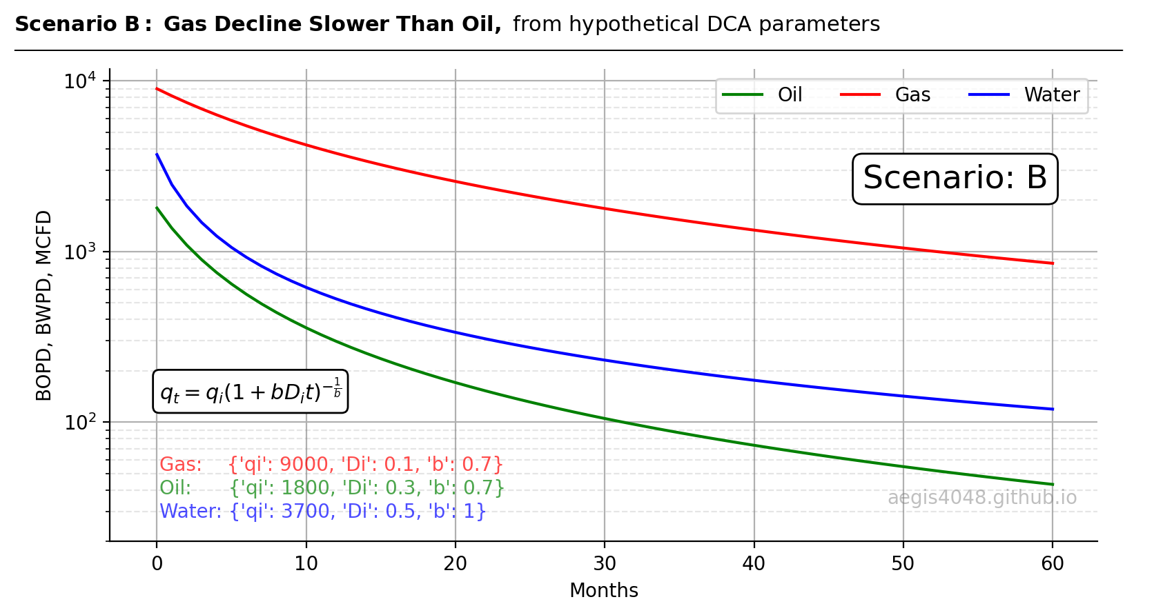
Figure 4: Well decline curve prediction from the DCA parameters in scenario B of Figure 2.
Source Code For Figure (4)
import pandas as pd
import numpy as np
import matplotlib.pyplot as plt


def general_decline(t, qi, Di, b):
    """
    Arps' decline equation for production decline modeling.

    Args:
        t (array-like): Time values.
        qi (float): Initial production rate.
        Di (float): Initial decline rate.
        b (float): Decline exponent.

    Returns:
        array-like: Production rate at time t.
    """
    return qi * (1 + b * Di * t) ** (-1 / b)

params = {
    'Oil': {'qi': 1800, 'Di': 0.3, 'b': .7},
    'Gas': {'qi': 9000, 'Di': 0.1, 'b': 0.7},
    'Water': {'qi': 3700, 'Di': 0.5, 'b': 1}
}

x = np.arange(0, 61)
fits = {
    'Oil': [],
    'Gas': [],
    'Water': [],
}
for key in params.keys():
    target_params = list(params[key].values())
    fits[key] = general_decline(x, *target_params)
df = pd.DataFrame.from_dict(fits)
df['Count'] = x

fig, ax = plt.subplots(figsize=(8, 4.5))

oc = 'green'
gc = 'red'
wc = 'blue'


ax.plot(df['Count'], df['Oil'], c=oc, label='Oil')
ax.plot(df['Count'], df['Gas'], c=gc, label='Gas')
ax.plot(df['Count'], df['Water'], c=wc, label='Water')


ax.set_xlabel('Months')
ax.set_ylabel('BOPD, BWPD, MCFD')


ax.grid(True)
ax.spines['top'].set_visible(False)
ax.spines['right'].set_visible(False)

#ax.minorticks_on()
ax.grid(axis='both', which='minor', color='grey', linestyle='--', alpha=0.2)
ax.legend(ncol=6, loc='upper right')

ymax = 10000
ymin = 10
xmax = ax.get_xlim()[1]
xmin = 0 - xmax * 0.05
ax.set_yscale('log')
ax.set_ylim(20, None)
ax.set_xlim(xmin, None)

ax.text(0.05, 0.15, 'Gas:    ' + str(params['Gas']), fontsize=10, ha='left', transform=ax.transAxes, color=gc, alpha=0.7)
ax.text(0.05, 0.1,  'Oil:      ' + str(params['Oil']), fontsize=10, ha='left', transform=ax.transAxes, color=oc, alpha=0.7)
ax.text(0.05, 0.05, 'Water: ' + str(params['Water']), fontsize=10, ha='left', transform=ax.transAxes, color=wc, alpha=0.7)

arps_equation = r"$q_t = q_i \left( 1 + b D_i t \right)^{-\frac{1}{b}}$"
ax.text(
    0.05, 0.35, arps_equation, fontsize=11, ha='left', va='top', transform=ax.transAxes, color='black',
    bbox=dict(facecolor='white', edgecolor='black', boxstyle='round,pad=0.3')
)

ax.text(
    0.95, 0.8, 'Scenario: B', fontsize=17, ha='right', va='top', transform=ax.transAxes, color='black',
    bbox=dict(facecolor='white', edgecolor='black', boxstyle='round,pad=0.3')
)

def setbold(txt):
    return ' '.join([r"$\bf{" + item + "}$" for item in txt.split(' ')])

bold_txt = setbold('Scenario B: Gas Decline Slower Than Oil, ')
plain_txt = 'from hypothetical DCA parameters'
fig.suptitle(bold_txt + plain_txt, verticalalignment='top', x=0, horizontalalignment='left', fontsize=11)
yloc = 0.9
ax.annotate('', xy=(0.01, yloc + 0.01), xycoords='figure fraction', xytext=(1.02, yloc + 0.01),
            arrowprops=dict(arrowstyle="-", color='k', lw=0.7))

ax.text(0.98, 0.08, 'aegis4048.github.io', fontsize=10, ha='right', transform=ax.transAxes, color='grey', alpha=0.5)

fig.tight_layout()
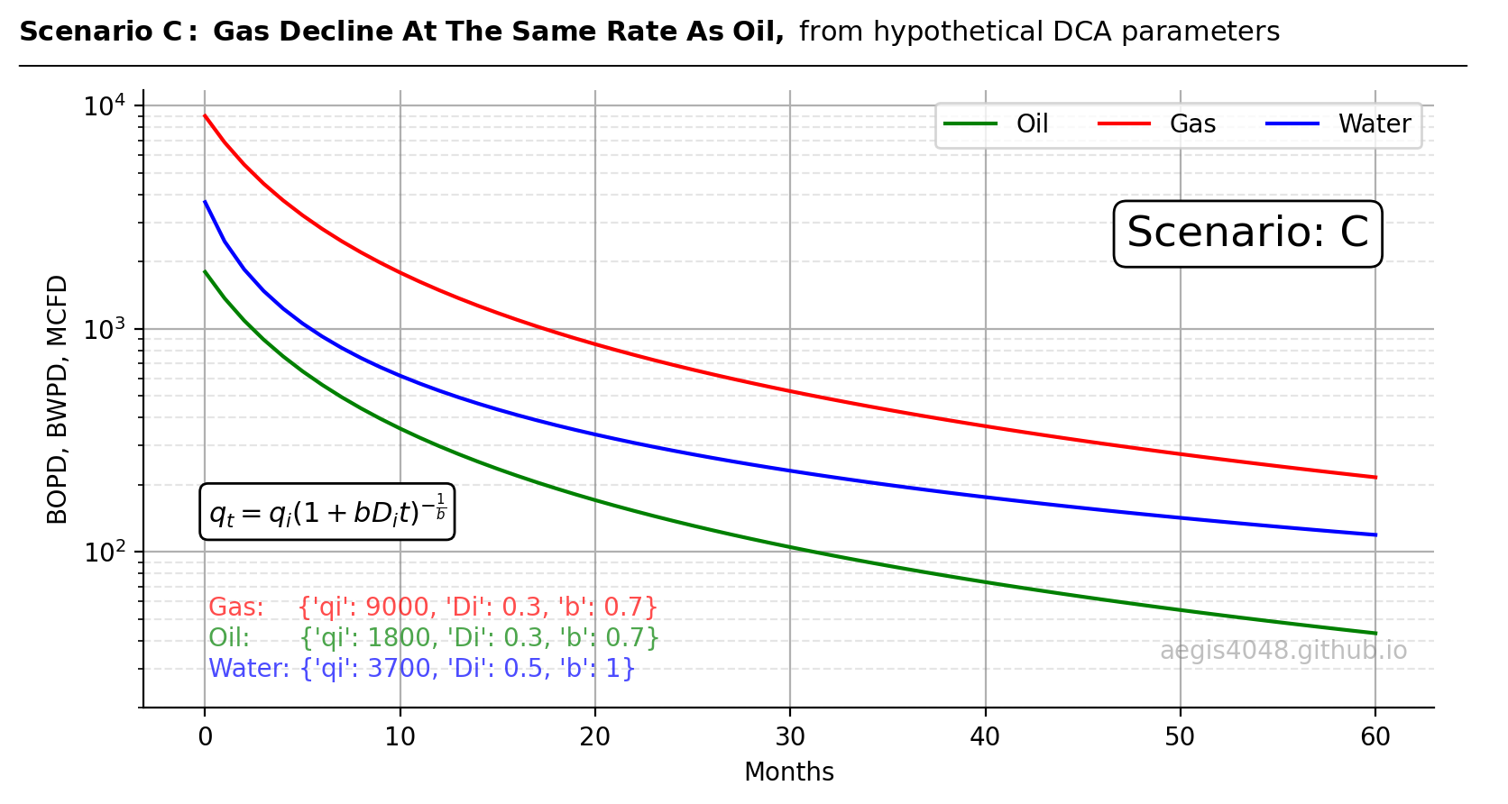
Figure 5: Well decline curve prediction from the DCA parameters in scenario C of Figure 2.
Source Code For Figure (5)
import pandas as pd
import numpy as np
import matplotlib.pyplot as plt


def general_decline(t, qi, Di, b):
    """
    Arps' decline equation for production decline modeling.

    Args:
        t (array-like): Time values.
        qi (float): Initial production rate.
        Di (float): Initial decline rate.
        b (float): Decline exponent.

    Returns:
        array-like: Production rate at time t.
    """
    return qi * (1 + b * Di * t) ** (-1 / b)

params = {
    'Oil': {'qi': 1800, 'Di': 0.3, 'b': .7},
    'Gas': {'qi': 9000, 'Di': 0.3, 'b': 0.7},
    'Water': {'qi': 3700, 'Di': 0.5, 'b': 1}
}

x = np.arange(0, 61)
fits = {
    'Oil': [],
    'Gas': [],
    'Water': [],
}
for key in params.keys():
    target_params = list(params[key].values())
    fits[key] = general_decline(x, *target_params)
df = pd.DataFrame.from_dict(fits)
df['Count'] = x

fig, ax = plt.subplots(figsize=(8, 4.5))

oc = 'green'
gc = 'red'
wc = 'blue'


ax.plot(df['Count'], df['Oil'], c=oc, label='Oil')
ax.plot(df['Count'], df['Gas'], c=gc, label='Gas')
ax.plot(df['Count'], df['Water'], c=wc, label='Water')


ax.set_xlabel('Months')
ax.set_ylabel('BOPD, BWPD, MCFD')


ax.grid(True)
ax.spines['top'].set_visible(False)
ax.spines['right'].set_visible(False)

#ax.minorticks_on()
ax.grid(axis='both', which='minor', color='grey', linestyle='--', alpha=0.2)
ax.legend(ncol=6, loc='upper right')

ymax = 10000
ymin = 10
xmax = ax.get_xlim()[1]
xmin = 0 - xmax * 0.05
ax.set_yscale('log')
ax.set_ylim(20, None)
ax.set_xlim(xmin, None)

ax.text(0.05, 0.15, 'Gas:    ' + str(params['Gas']), fontsize=10, ha='left', transform=ax.transAxes, color=gc, alpha=0.7)
ax.text(0.05, 0.1,  'Oil:      ' + str(params['Oil']), fontsize=10, ha='left', transform=ax.transAxes, color=oc, alpha=0.7)
ax.text(0.05, 0.05, 'Water: ' + str(params['Water']), fontsize=10, ha='left', transform=ax.transAxes, color=wc, alpha=0.7)

arps_equation = r"$q_t = q_i \left( 1 + b D_i t \right)^{-\frac{1}{b}}$"
ax.text(
    0.05, 0.35, arps_equation, fontsize=11, ha='left', va='top', transform=ax.transAxes, color='black',
    bbox=dict(facecolor='white', edgecolor='black', boxstyle='round,pad=0.3')
)

ax.text(
    0.95, 0.8, 'Scenario: C', fontsize=17, ha='right', va='top', transform=ax.transAxes, color='black',
    bbox=dict(facecolor='white', edgecolor='black', boxstyle='round,pad=0.3')
)


def setbold(txt):
    return ' '.join([r"$\bf{" + item + "}$" for item in txt.split(' ')])

bold_txt = setbold('Scenario C: Gas Decline At The Same Rate As Oil, ')
plain_txt = 'from hypothetical DCA parameters'
fig.suptitle(bold_txt + plain_txt, verticalalignment='top', x=0, horizontalalignment='left', fontsize=11)
yloc = 0.9
ax.annotate('', xy=(0.01, yloc + 0.01), xycoords='figure fraction', xytext=(1.02, yloc + 0.01),
            arrowprops=dict(arrowstyle="-", color='k', lw=0.7))

ax.text(0.98, 0.08, 'aegis4048.github.io', fontsize=10, ha='right', transform=ax.transAxes, color='grey', alpha=0.5)

fig.tight_layout()
2.3. Simulation results
BR&E Promax is used to simulate flash gas declines at the heater and VRT. The base model shown in Figure 1 was fed with the three declining scenarios shown in Figures 3, 4, and 5. Declines up to 60 months are simulated. The simulaion results are shown in Table 1 and Table 2 below. Not all months are shown for brevity. You can download the full Simulation Results Data (VRU_Declining_Economics-Sim_Results.xlsx) to review the complete Promax simulation results in Excel. Refer to Tabs "1a", "1b", and "1c". Note that the DCA parameters shown on the right are realistic parameters that can be observed in the field.
Results Summary
Flash gas declines closely follow the oil decline, with gas declines having a relatively minor impact in comparison.
The primary driver of downstream flash gas rate declines is the oil production rate. Do not predict flash gas decline from the produced (sales) gas decline.
VRU flowrates can decrease by up to 86% compared to IP flowrates in 12 months, or more than 50% in just 3 months. They decline faster than expected, much like oil production.
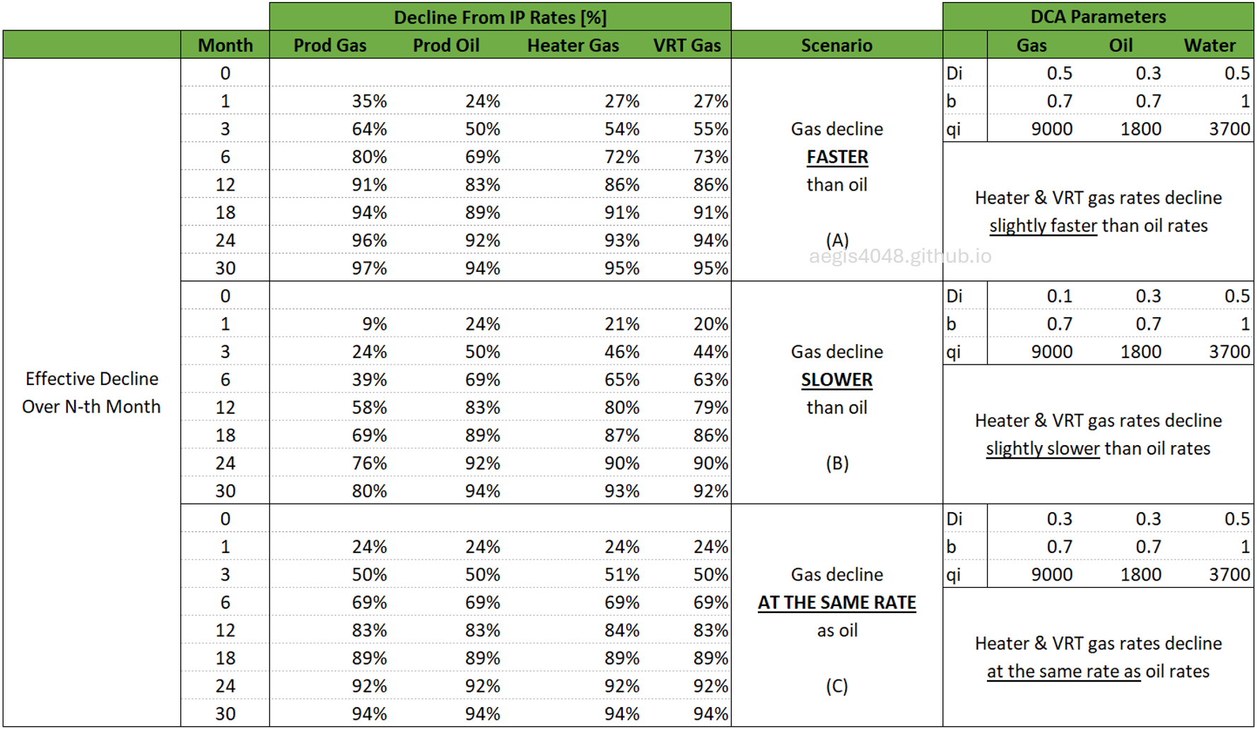
Table 1: Simulation results using the base model shown in Figure 1 and declining flowrate inputs shown in Figures 3, 4, and 5. The DCA parameters shown on the right represents declining scenarios used to simulate well decline. The percentages represent how much production declines compared to the initial production. Actual flowrate numbers are shown in Table 2 below. The first rows in each scenario are emtpy because there's no decline at month=0.
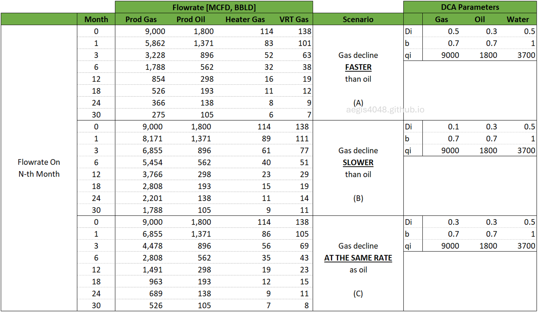
Table 2: Simulation results using the base model shown in Figure 1 and declining flowrate inputs shown in Figures 3, 4, and 5. The DCA parameters shown on the right represents declining scenarios used to simulate well decline.
3. VRU Economics
VRU economics are calculated based on the simulation results from scenario C in Table 2 for both the heater treater and VRT. The calculation tables are provided below in Table 3 for the VRU installation on the VRT and Table 4 for the VRU installation on the heater. Note that the energy content of the flash gas from the VRT (2690 Btu/scf) is higher than that from the heater (1930 Btu/scf). This is because lighter hydrocarbons like methane and ethane flash off at higher pressures, while heavier hydrocarbons do not flash until the pressure is significantly lower. Recall from the site setups in Section 2.1 that the heater operates at 50 psig, while the VRT operates at 3 psig.
You can download the full Simulation Results Data (VRU_Declining_Economics-Sim_Results.xlsx) to review the economics calculation formulas in Excel. Refer to Tabs "Gas Economics Calcualtor - HT", and "Gas Economics Calcualtor - VRT".
Assumptions
- Oklahoma 7% sales gas tax.
- $0.75/MCF gathering fee, typical for Oklahoma.
- Separate VRUs are used for heater and VRT each. This is because compressor inlet cannot take gases from two different pressures (the compressor company I work for has "Multi-stream" technology that enables dual inlet for two pressures, but it's not the focus of this article. Contact me if you are interested).
- Same VRU sizing for both VRT and heater (although the heater may require smaller sizing due to its lower flash gas flowrate and higher operating pressure. The higher the gas pressure at the compressor inlet, the greater the compressor's flowrate capacity).
- Generic $3,500 monthly VRU rental cost. This can vary depending on application and vendors.
- The operator is paid based on energy content (MMBtu) rather than volume. This may not be an option for some regions.
- 30 days assumed for all months for calculation simplicity.
Economics Summary
VRU installation on the heater becomes uneconomical after month 8.
VRU installation on the VRT becomes uneconomical after month 15.
The heater application becomes uneconomical much faster than the VRT due to its lower flowrate (22% lower) and lower energy content (39% lower).
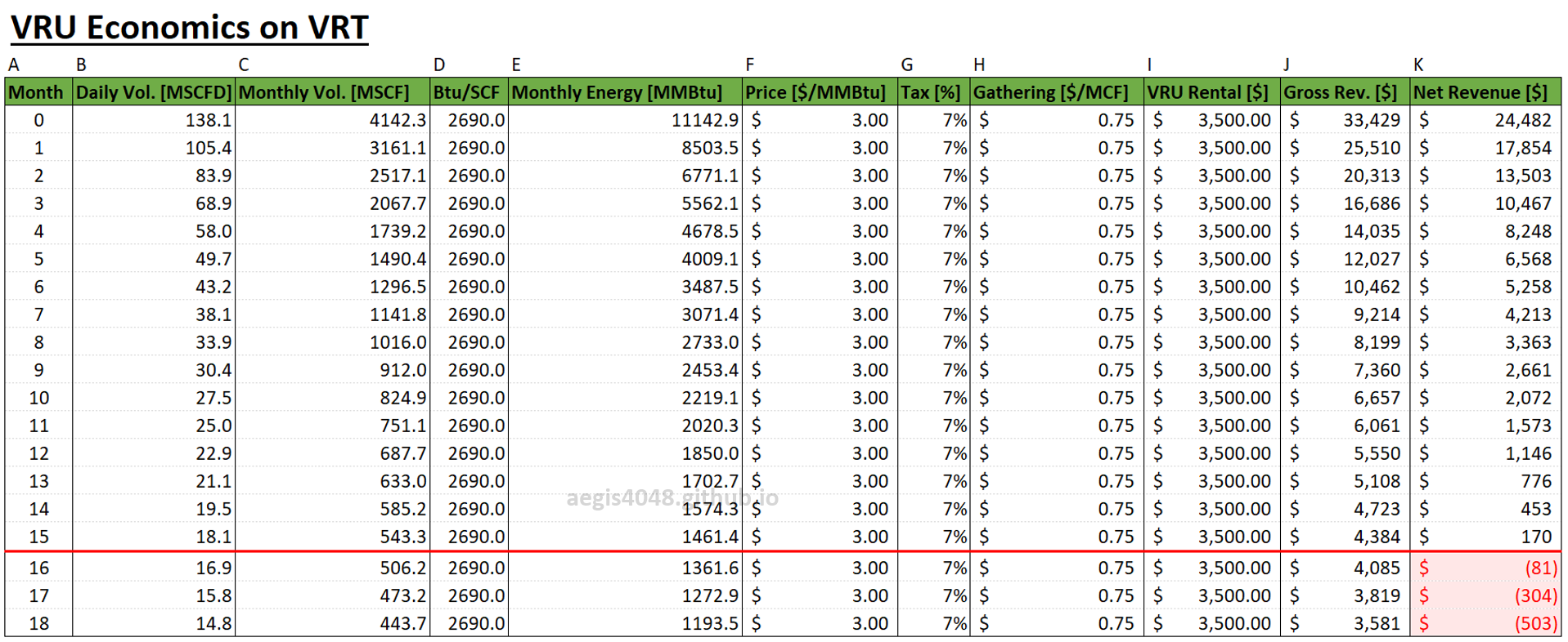
Table 3: VRU economics calculation table for VRU installed on scenario C's VRT gas rates. The VRU becomes uneconomical after month 15.
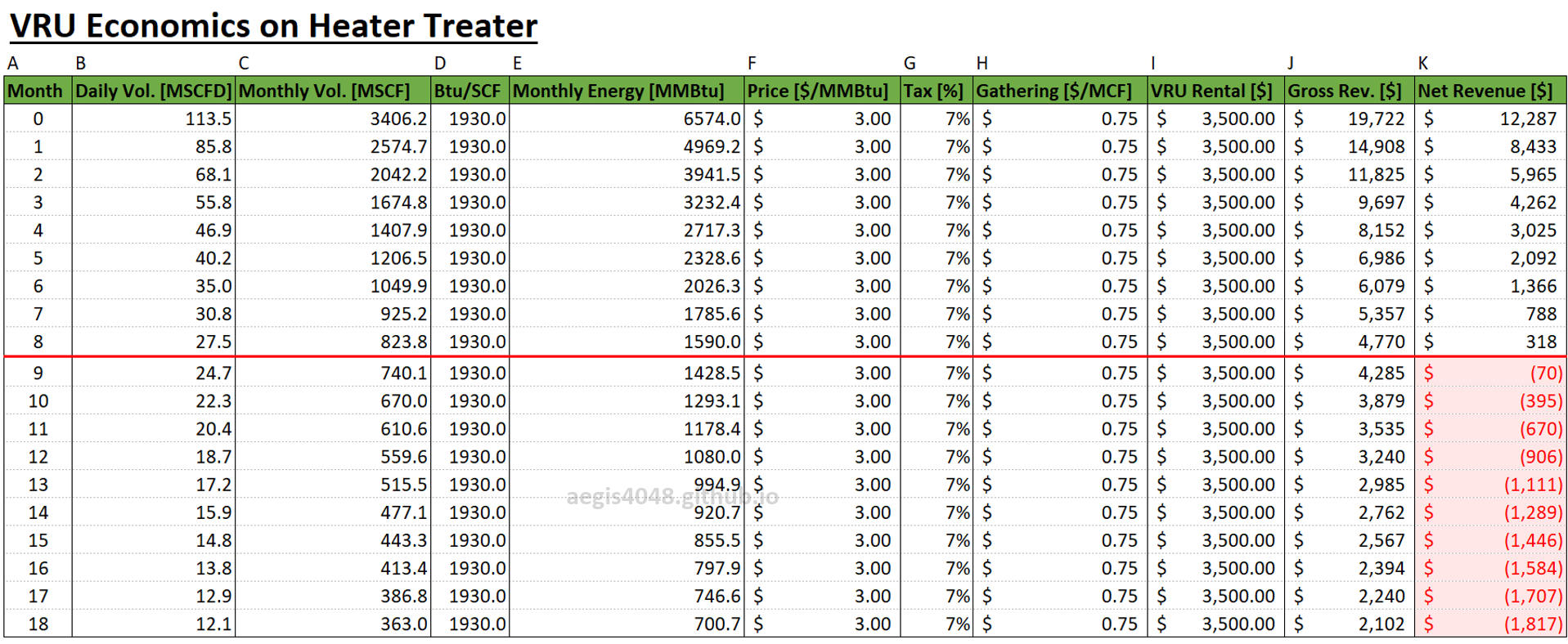
Table 4: VRU economics calculation table for VRU installed on scenario C's heater gas rates. The VRU becomes uneconomical after month 8. VRU installation on heater becomes uneconomical much faster than VRT application due to heater gas having lower flowrate and lower energy content.
4. Conclusion/Summary
1. Flash gas rates for VRU applications may decline quickly, quicker than people think. They follow the oil decline curve.
2. Many people in the industry tend to forget about the fact that VRU flowrates decline quickly. I've witnessed this first-hand working at a compressor company. Downsizing is often not done in a timely manner. This is because VRU is not their primary concern most of the time.
3. Process simulations are performed to show the impact of oil and gas decline on downstream flash gases from low pressure vessels. Simulation site setups are described in Section 2.1. Well declining rates are simulated with 3 sets of DCA parameters described in Section 2.2.
4. Simulation results in Table 1 indicate that flash gas rates at low pressure vessels (heater, VRT) follow oil decline. The primary sales gas has some impact, but negligible compared to oil decline's influence.
5. When forecasting VRU decline, use the decline rate of oil production. Do not predict off the primary produced gas decline.
6. Flash gas rates decline quickly after IP, just like oil. In Table 1, flash gas off the heater became halved in 3 months, and quartered in 6 months.
7. Due to fast decline after the initial production, VRU may become quickly uneconomical. In Table 4 that shows VRU economics for heater, VRU installation on heater flash gas became uneconomical 8 months after IP. Failure to downsize the unit in a timely manner, or being stuck with a long-term contract (unless the unit can be moved to another pad) can be detrimental to lease operating expense (LOE).
8. Be careful when signing a long-term contract for VRUs. Be prepared to predict VRU economics and move the long-term contracted VRU to new locations on a timely manner to avoid economic loss.
9. Energy content coming from low pressure vessel (VRT @3#: 2690 Btu/scf) is higher than the one coming from higher pressure vessel (Heater @50#: 1930 Btu/scf). This is because lighter hydrocarbons like methane and ethane flash off at higher pressures, while heavier hydrocarbons do not flash until the pressure is significantly lower. The difference in energy content has a huge impact on VRU economics. Process simulations are required for accurate prediction of flash gas energy content at different vessels.
Contact me via email (aegis4048@gmail.com) or leave a comment below for any professional inquiries regarding compressor applications or process simulations.
Related Posts
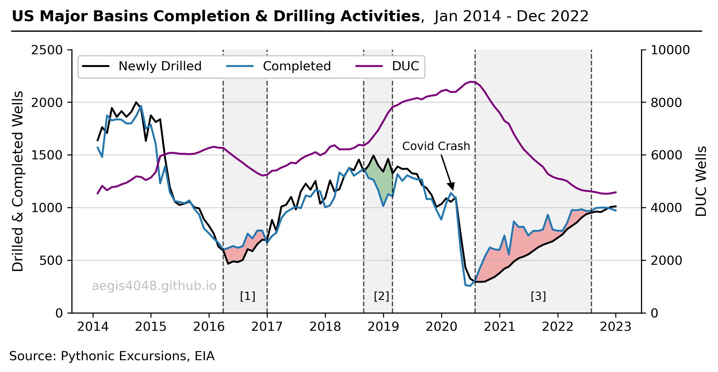
DUC Wells and Their Economic Complications
During the Covid-19 Pandemic, the operators opted not to drill new wells, but instead completed their existing DUC wells to meet demand while conserving cash. This post explains the concept and the economic impact of DUC wells on the US energy industry.
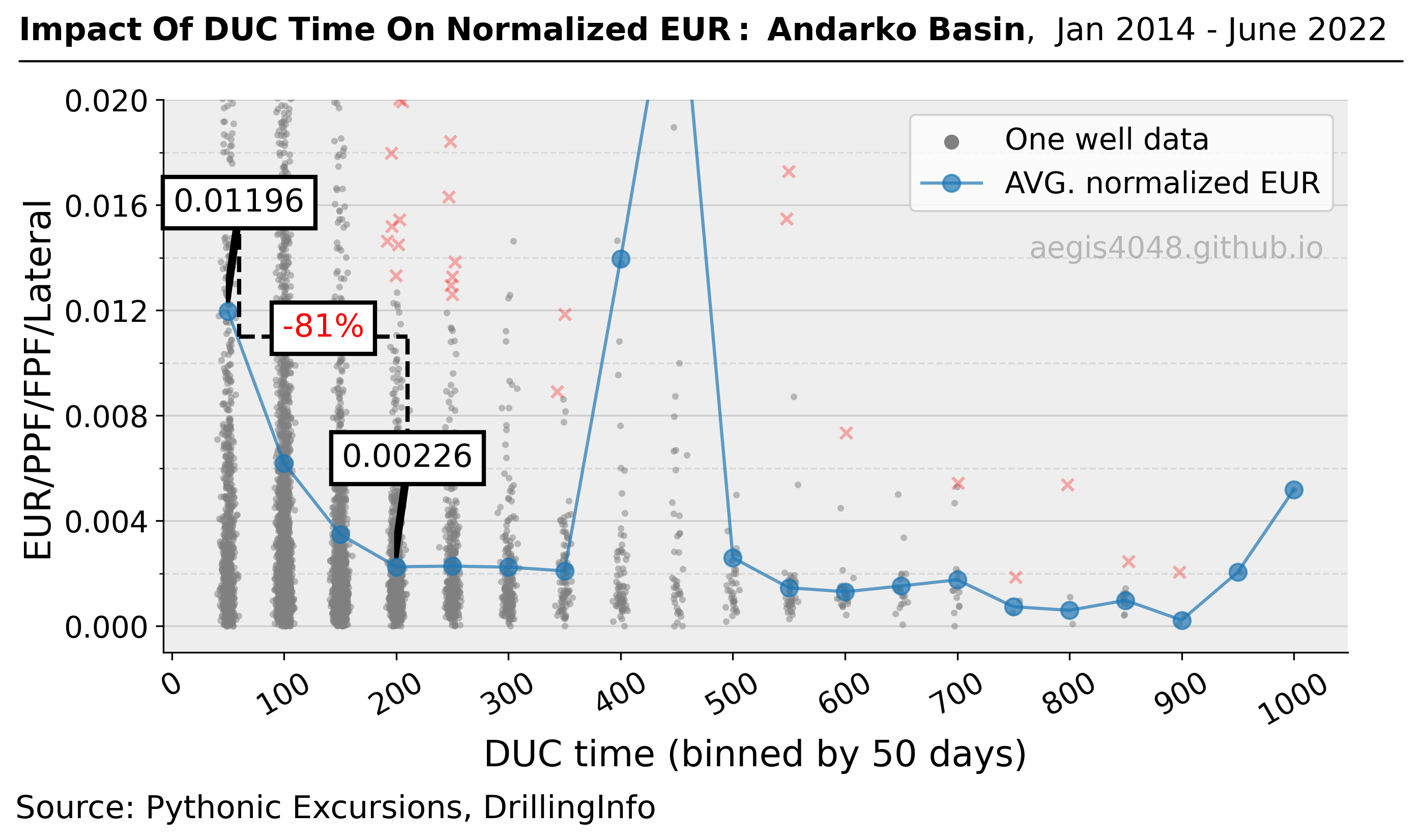
Quantifying The Impact Of Completion Delay Since Drilled On Production
In times of unfavorable commodity prices, operators may delay completion after drilling in the hope of a price recovery. The study conducted in this article shows why this may not be a financially sound idea for certain basins by quantifying the impact of DUC time on normalized EURs.
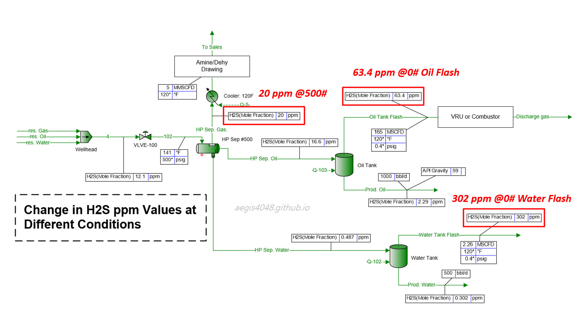
H₂S Levels: Why High-Pressure Samples Don't Tell the Full Story
H₂S ppm levels obtained from high pressure applications (HP separators) are often re-used for low pressure applications (atmospheric tanks). H₂S levels soar 3~25 times at low pressures. This post explains the thermodynamics behind H2S ppm level variations and provide simulation results summary for practical applications.
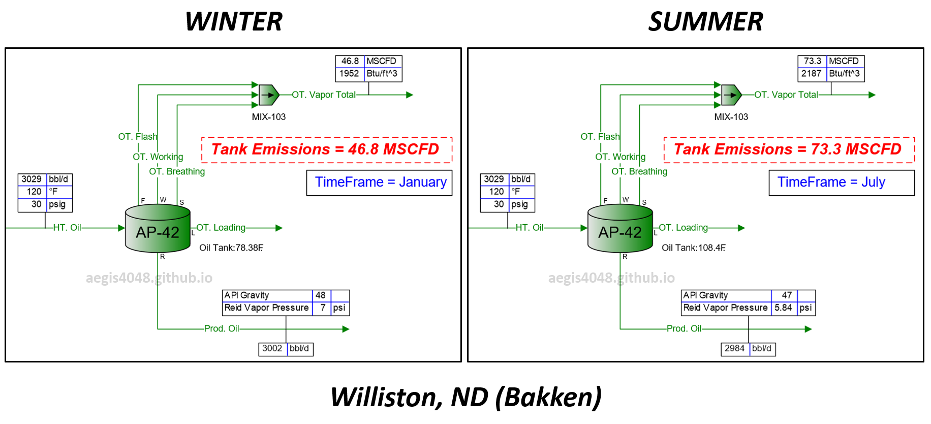
Impact of Seasonal Changes on Storage Tank Emissions
Storage tank temperatures rise in summer due to hot air, leading to higher emission volumes compared to winter. This temperature increase also impacts the dew point T, SG, and energy content (Btu/scf) of tank vapor. This post explains the phase behavior changes due to temperature shifts and provides a summary table with recommended operating capacity margins for emission handling systems across various regions.
Operation of Oil-Flooded Screw Compressor Explained
A detailed guide to oil-flooded screw compressor operations, covering compressor characteristics, operating capacity, unit P&ID, blowcase systems, control device mechanisms (valves and switches), pressure and temperature control, recycle mode, surface facility P&ID applications, lube oil contamination issues, electric vs. gas engine model comparisons, and more.