Multiple Linear Regression and Visualization in Python
Category > Machine Learning
Nov 18, 2019There are many advanced machine learning methods with robust prediction accuracy. While complex models may outperform simple models in predicting a response variable, simple models are better for understanding the impact & importance of each feature on a response variable. When the task at hand can be described by a linear model, linear regression triumphs over all other machine learning methods in feature interpretation due to its simplicity.
This post attempts to help your understanding of linear regression in multi-dimensional feature space, model accuracy assessment, and provide code snippets for multiple linear regression in Python.
0. Sample data description
We will use one sample data throughout this post. The sample data is relevant to the oil & gas industry. It is originally from Dr. Michael Pyrcz, petroleum engineering professor at the University of Texas at Austin. The original data can be found from his github repo. You can also use direct download, or directly access it using pandas url like below:
import pandas as pd

file = 'https://aegis4048.github.io/downloads/notebooks/sample_data/unconv_MV_v5.csv'
df = pd.read_csv(file)
df.head(10)
Description of headers
- Well : well index
- Por : well average porosity (%)
- Perm : permeability (mD)
- AI : accoustic impedance (kg/m2s*10^6)
- Brittle : brittleness ratio (%)
- TOC : total organic carbon (%)
- VR : vitrinite reflectance (%)
- Prod : gas production per day (MCFD) - Response Variable
We have six features (Por, Perm, AI, Brittle, TOC, VR) to predict the response variable (Prod). Based on the permutation feature importances shown in figure (1), Por is the most important feature, and Brittle is the second most important feature.
Permutation feature ranking is out of the scope of this post, and will not be discussed in detail. Feature importances are obtained with rfpimp python library. For more information about permutation feature ranking, refer to this article: Beware Default Random Forest Importances
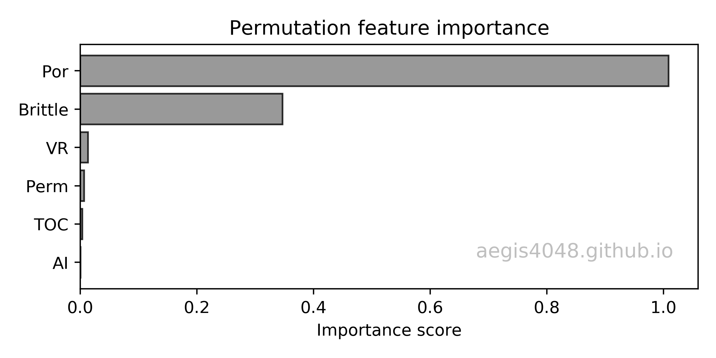
Figure 1: Permutation feature ranking
Source Code For Figure (1)
                import rfpimp
                import pandas as pd
                import numpy as np
                from sklearn.ensemble import RandomForestRegressor
                from sklearn.model_selection import train_test_split

                ######################################## Data preparation #########################################

                file = 'https://aegis4048.github.io/downloads/notebooks/sample_data/unconv_MV_v5.csv'
                df = pd.read_csv(file)
                features = ['Por', 'Perm', 'AI', 'Brittle', 'TOC', 'VR', 'Prod']

                ######################################## Train/test split #########################################

                df_train, df_test = train_test_split(df, test_size=0.20)
                df_train = df_train[features]
                df_test = df_test[features]

                X_train, y_train = df_train.drop('Prod',axis=1), df_train['Prod']
                X_test, y_test = df_test.drop('Prod',axis=1), df_test['Prod']

                ################################################ Train #############################################

                rf = RandomForestRegressor(n_estimators=100, n_jobs=-1)
                rf.fit(X_train, y_train)

                ############################### Permutation feature importance #####################################

                imp = rfpimp.importances(rf, X_test, y_test)

                ############################################## Plot ################################################

                fig, ax = plt.subplots(figsize=(6, 3))

                ax.barh(imp.index, imp['Importance'], height=0.8, facecolor='grey', alpha=0.8, edgecolor='k')
                ax.set_xlabel('Importance score')
                ax.set_title('Permutation feature importance')
                ax.text(0.8, 0.15, 'aegis4048.github.io', fontsize=12, ha='center', va='center',
                        transform=ax.transAxes, color='grey', alpha=0.5)
                plt.gca().invert_yaxis()

                fig.tight_layout()
1. Multiple linear regression
Multiple linear regression model has the following structure:
Bivarate linear regression model (that can be visualized in 2D space) is a simplification of eq (1). Bivariate model has the following structure:
A picture is worth a thousand words. Let's try to understand the properties of multiple linear regression models with visualizations. First, 2D bivariate linear regression model is visualized in figure (2), using Por as a single feature. Although porosity is the most important feature regarding gas production, porosity alone captured only 74% of variance of the data.
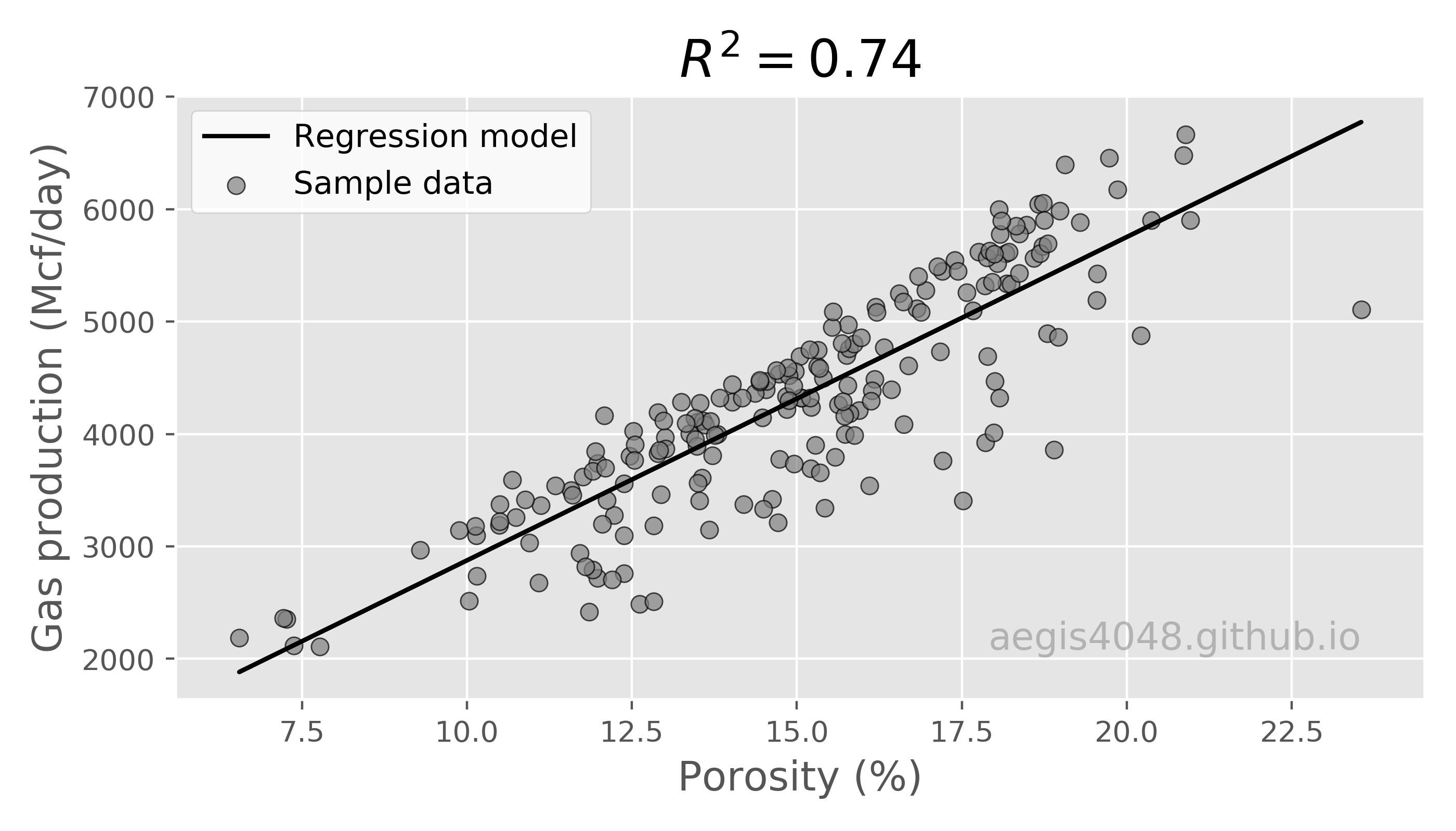
Figure 2: 2D Linear regression model
Source Code For Figure (2)
                import pandas as pd
                import matplotlib.pyplot as plt
                from sklearn import linear_model

                ######################################## Data preparation #########################################

                file = 'https://aegis4048.github.io/downloads/notebooks/sample_data/unconv_MV_v5.csv'
                df = pd.read_csv(file)

                X = df['Por'].values.reshape(-1,1)
                y = df['Prod'].values

                ################################################ Train #############################################

                ols = linear_model.LinearRegression()
                model = ols.fit(X, y)
                response = model.predict(X)

                ############################################## Evaluate ############################################

                r2 = model.score(X, y)

                ############################################## Plot ################################################

                plt.style.use('default')
                plt.style.use('ggplot')

                fig, ax = plt.subplots(figsize=(8, 4))

                ax.plot(X, response, color='k', label='Regression model')
                ax.scatter(X, y, edgecolor='k', facecolor='grey', alpha=0.7, label='Sample data')
                ax.set_ylabel('Gas production (Mcf/day)', fontsize=14)
                ax.set_xlabel('Porosity (%)', fontsize=14)
                ax.text(0.8, 0.1, 'aegis4048.github.io', fontsize=13, ha='center', va='center',
                         transform=ax.transAxes, color='grey', alpha=0.5)
                ax.legend(facecolor='white', fontsize=11)
                ax.set_title('$R^2= %.2f$' % r2, fontsize=18)

                fig.tight_layout()
How would the model look like in 3D space? Let's take a look at figure (3). Due to the 3D nature of the plot, multiple plots were generated from different angles. Two features (Por and Brittle) were used to predict the response variable Prod. With the help of the additional feature Brittle, the linear model experience significant gain in accuracy, now capturing 93% variability of data.
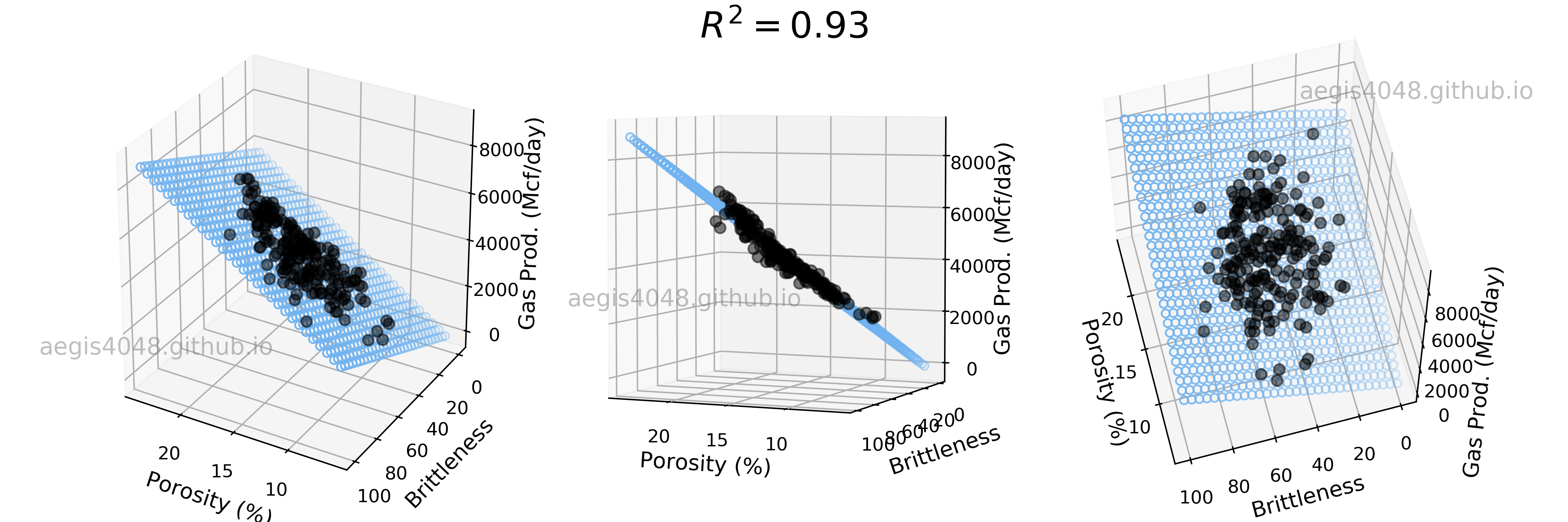
Figure 3: 3D Linear regression model with strong features
Source Code For Figure (3)
                import pandas as pd
                import numpy as np
                import matplotlib.pyplot as plt
                from sklearn import linear_model
                from mpl_toolkits.mplot3d import Axes3D

                ######################################## Data preparation #########################################

                file = 'https://aegis4048.github.io/downloads/notebooks/sample_data/unconv_MV_v5.csv'
                df = pd.read_csv(file)

                X = df[['Por', 'Brittle']].values.reshape(-1,2)
                Y = df['Prod']

                ######################## Prepare model data point for visualization ###############################

                x = X[:, 0]
                y = X[:, 1]
                z = Y

                x_pred = np.linspace(6, 24, 30)   # range of porosity values
                y_pred = np.linspace(0, 100, 30)  # range of brittleness values
                xx_pred, yy_pred = np.meshgrid(x_pred, y_pred)
                model_viz = np.array([xx_pred.flatten(), yy_pred.flatten()]).T

                ################################################ Train #############################################

                ols = linear_model.LinearRegression()
                model = ols.fit(X, Y)
                predicted = model.predict(model_viz)

                ############################################## Evaluate ############################################

                r2 = model.score(X, Y)

                ############################################## Plot ################################################

                plt.style.use('default')

                fig = plt.figure(figsize=(12, 4))

                ax1 = fig.add_subplot(131, projection='3d')
                ax2 = fig.add_subplot(132, projection='3d')
                ax3 = fig.add_subplot(133, projection='3d')

                axes = [ax1, ax2, ax3]

                for ax in axes:
                    ax.plot(x, y, z, color='k', zorder=15, linestyle='none', marker='o', alpha=0.5)
                    ax.scatter(xx_pred.flatten(), yy_pred.flatten(), predicted, facecolor=(0,0,0,0), s=20, edgecolor='#70b3f0')
                    ax.set_xlabel('Porosity (%)', fontsize=12)
                    ax.set_ylabel('Brittleness', fontsize=12)
                    ax.set_zlabel('Gas Prod. (Mcf/day)', fontsize=12)
                    ax.locator_params(nbins=4, axis='x')
                    ax.locator_params(nbins=5, axis='x')

                ax1.text2D(0.2, 0.32, 'aegis4048.github.io', fontsize=13, ha='center', va='center',
                           transform=ax1.transAxes, color='grey', alpha=0.5)
                ax2.text2D(0.3, 0.42, 'aegis4048.github.io', fontsize=13, ha='center', va='center',
                           transform=ax2.transAxes, color='grey', alpha=0.5)
                ax3.text2D(0.85, 0.85, 'aegis4048.github.io', fontsize=13, ha='center', va='center',
                           transform=ax3.transAxes, color='grey', alpha=0.5)

                ax1.view_init(elev=28, azim=120)
                ax2.view_init(elev=4, azim=114)
                ax3.view_init(elev=60, azim=165)

                fig.suptitle('$R^2 = %.2f$' % r2, fontsize=20)

                fig.tight_layout()
How would the 3D linear model look like if less powerful features are selected? Let's choose Por and VR as our new features and fit a linear model. In figure (4) below, we see that R-squared decreased compared to figure (3) above. The effect of decreased model performance can be visually observed by comparing their middle plots; the scatter plots in figure (3) are more densely populated around the 2D model plane than the scatter plots in figure (4).
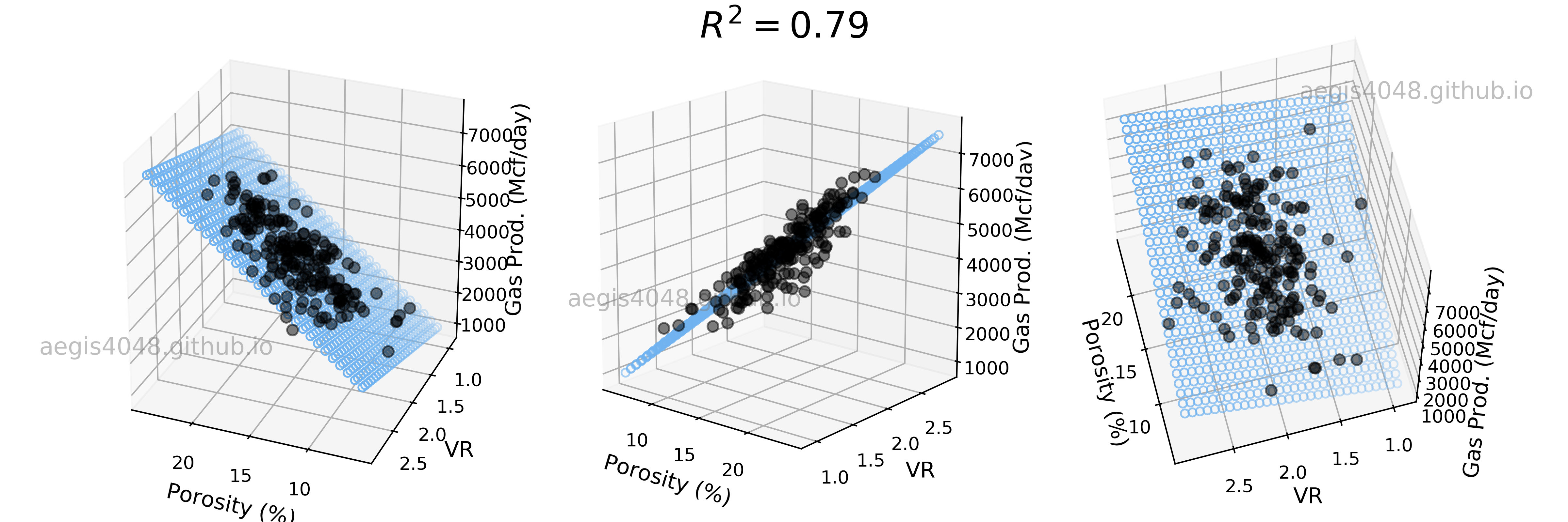
Figure 4: 3D Linear regression model with weak features
Source Code For Figure (4)
                import pandas as pd
                import numpy as np
                import matplotlib.pyplot as plt
                from sklearn import linear_model
                from mpl_toolkits.mplot3d import Axes3D

                ######################################## Data preparation #########################################

                file = 'https://aegis4048.github.io/downloads/notebooks/sample_data/unconv_MV_v5.csv'
                df = pd.read_csv(file)

                X = df[['Por', 'VR']].values.reshape(-1,2)
                Y = df['Prod']

                ######################## Prepare model data point for visualization ###############################

                x = X[:, 0]
                y = X[:, 1]
                z = Y

                x_pred = np.linspace(6, 24, 30)      # range of porosity values
                y_pred = np.linspace(0.93, 2.9, 30)  # range of VR values
                xx_pred, yy_pred = np.meshgrid(x_pred, y_pred)
                model_viz = np.array([xx_pred.flatten(), yy_pred.flatten()]).T

                ################################################ Train #############################################

                ols = linear_model.LinearRegression()
                model = ols.fit(X, Y)
                predicted = model.predict(model_viz)

                ############################################## Evaluate ############################################

                r2 = model.score(X, Y)

                ############################################## Plot ################################################

                plt.style.use('default')

                fig = plt.figure(figsize=(12, 4))

                ax1 = fig.add_subplot(131, projection='3d')
                ax2 = fig.add_subplot(132, projection='3d')
                ax3 = fig.add_subplot(133, projection='3d')

                axes = [ax1, ax2, ax3]

                for ax in axes:
                    ax.plot(x, y, z, color='k', zorder=15, linestyle='none', marker='o', alpha=0.5)
                    ax.scatter(xx_pred.flatten(), yy_pred.flatten(), predicted, facecolor=(0,0,0,0), s=20, edgecolor='#70b3f0')
                    ax.set_xlabel('Porosity (%)', fontsize=12)
                    ax.set_ylabel('VR', fontsize=12)
                    ax.set_zlabel('Gas Prod. (Mcf/day)', fontsize=12)
                    ax.locator_params(nbins=4, axis='x')
                    ax.locator_params(nbins=5, axis='x')

                ax1.text2D(0.2, 0.32, 'aegis4048.github.io', fontsize=13, ha='center', va='center',
                           transform=ax1.transAxes, color='grey', alpha=0.5)
                ax2.text2D(0.3, 0.42, 'aegis4048.github.io', fontsize=13, ha='center', va='center',
                           transform=ax2.transAxes, color='grey', alpha=0.5)
                ax3.text2D(0.85, 0.85, 'aegis4048.github.io', fontsize=13, ha='center', va='center',
                           transform=ax3.transAxes, color='grey', alpha=0.5)

                ax1.view_init(elev=27, azim=112)
                ax2.view_init(elev=16, azim=-51)
                ax3.view_init(elev=60, azim=165)

                fig.suptitle('$R^2 = %.2f$' % r2, fontsize=20)

                fig.tight_layout()
The full-rotation view of linear models are constructed below in a form of gif. Notice that the blue plane is always projected linearly, no matter of the angle. This is the reason that we call this a multiple "LINEAR" regression model. The model will always be linear, no matter of the dimensionality of your features. When you have more than 3 features, the model will be very difficult to be visualized, but you can expect that high dimensional linear models will also exhibit linear trend within their feature space.
Figure 5: Porosity and Brittleness Linear model GIF
Figure 6: Porosity and VR Linear model GIF
The gif was generated by creating 360 different plots viewed from different angles with the following code snippet, and combined into a single gif from imgflip.
for ii in np.arange(0, 360, 1):
    ax.view_init(elev=32, azim=ii)
    fig.savefig('gif_image%d.png' % ii)
Notes: Data encoding - regression with categorical variables
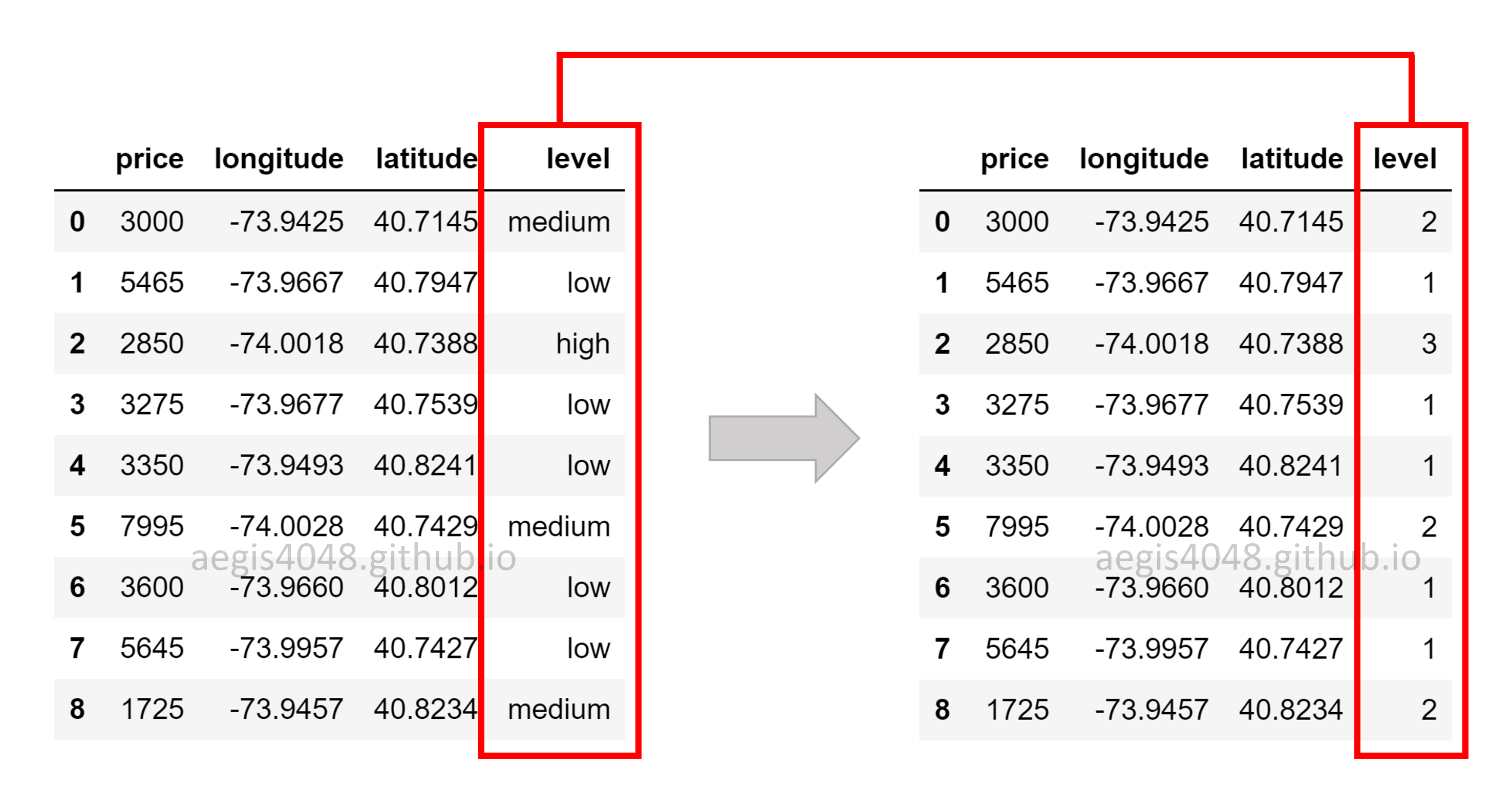
Regression requires features to be continuous. What happens if you have categorical features that are important? Do you have to ignore categorical variables, and run regression only with continuous variables? We can encode categorical variables into numerical variables to avoid this issue. Take a look at the below figure. The feature level was originally a categorial variable with three categories of ordinality. This means that there are hierarchy among the categories (ex: low < medium < high), and that their encoding needs to capture their ordinality. It is achieved by converting them in to 1, 2, and 3. This kind of encoding is called integer encoding
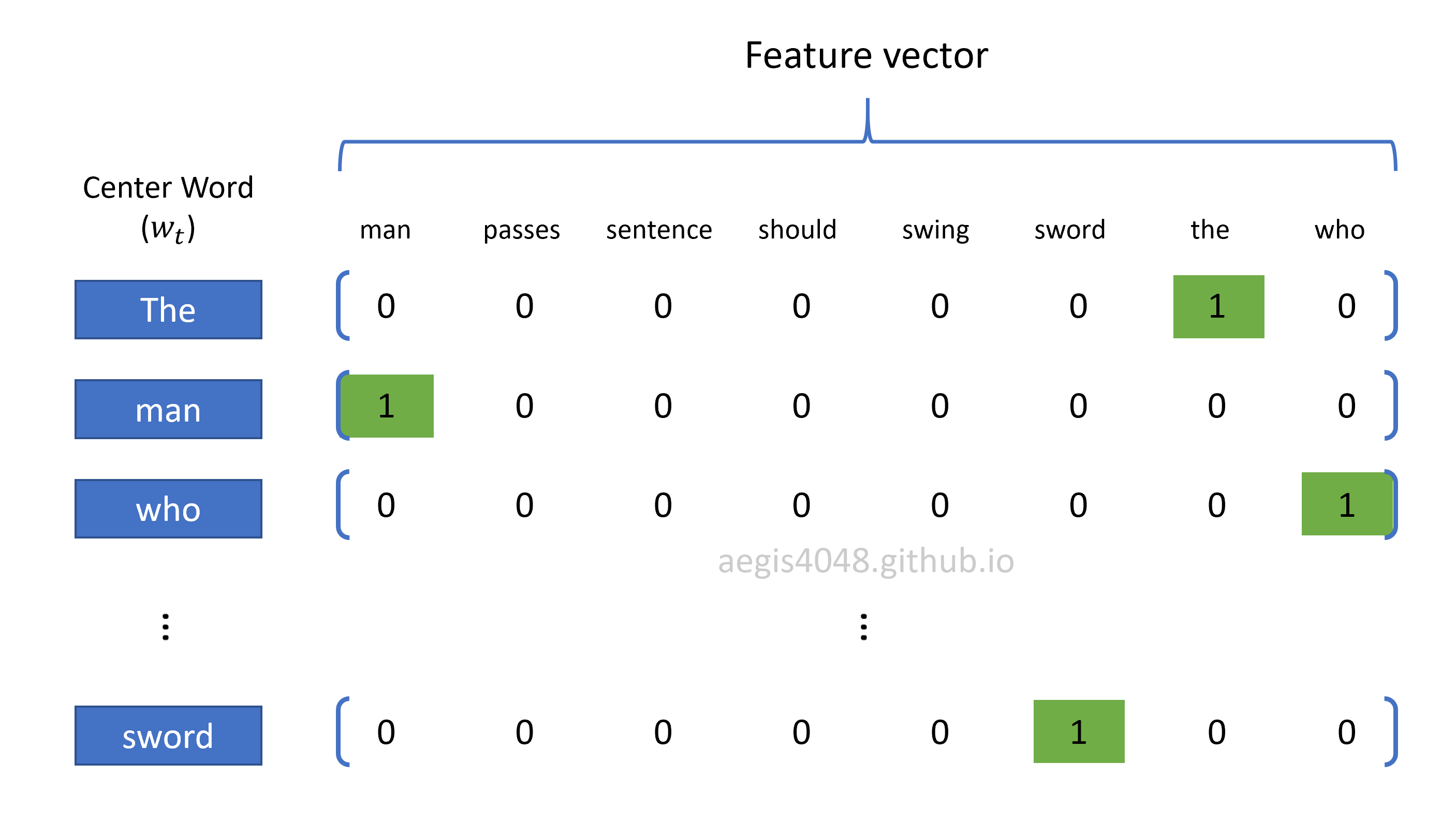
What if there are no ordinality among the categories of a feature? Then we use a technique called one-hot encoding to prevent a model from assuming natural ordering among categories that may suffer from model bias. Instead of using integer variables, we use binary variables. 1 indicates that the sample data falls into the specified category, while 0 indicates the otherwise. One-hot encoding is used in almost all natural languages problems, because vocabularies do not have ordinal relationships among themselves.
Pythonic Tip: 2D linear regression with scikit-learn
Linear regression is implemented in scikit-learn with sklearn.linear_model (check the documentation). For code demonstration, we will use the same oil & gas data set described in Section 0: Sample data description above.
Data prepration
First, import modules and data. We will use a single feature: Por. Response variable is Prod.
import pandas as pd
from sklearn import linear_model
import numpy as np

file = 'https://aegis4048.github.io/downloads/notebooks/sample_data/unconv_MV_v5.csv'
df = pd.read_csv(file)
Preprocess
If you get error messages like ValueError: Expected 2D array, got 1D array instead: ..., its the issue of preprocessing. Most scikit-learn training functions require reshape of features, such as reshape(-1, len(features)). In case you import data from Pandas dataframe, the first argument is always -1, and the second argument is the number of features, in a form of an integer. This preprocessing will also be required when you make predictions based on the fitted model later.
Check the shape of your features and response variable if you are experiencing errors.
import numpy as np

features = ['Por']
target = 'Prod'

X = df[features].values.reshape(-1, len(features))
y = df[target].values
print(X.shape)
print(y.shape)
Fit linear model
Since we have only one feature, the linear model we want to fit has the following structure:
Let's find out the values of $\beta_1$ (regression coefficient) and $\beta_2$ (y-intercept). Just like many other scikit-learn libraries, you instantiate the training model object with linear_model.LinearRegression(), and than fit the model with the feature X and the response variable y.
Note that ols stands for Ordinary Least Squares.
from sklearn import linear_model

ols = linear_model.LinearRegression()
model = ols.fit(X, y)
The linear regression coefficient can be accessed in a form of class attribute with model.coef_
model.coef_
The y-intercept can be accessed in a form of class attribute with model.intercept_
model.intercept_
Based on the result of the fit, we conclude that the gas production can be predicted from porosity, with the following linear model:
Accuracy assessment: $R^2$
How good was your model? You can evaluate your model performance in a form of R-squared, with model.score(X, y). X is the features, and y is the response variable used to fit the model.
model.score(X, y)
Make future prediction
Scikit-learn supports making predictions based on the fitted model with model.predict(X) method. X is a feature that requires preprocessing explained above. Recall that we used only one feature, and that len(features) = 1.
Let's say that you want to predict gas production when porosity is 15%. Then:
x_pred = np.array([15])
x_pred = x_pred.reshape(-1, len(features))  # preprocessing required by scikit-learn functions
model.predict(x_pred)
According to the model, gas production = 4313 Mcf/day when porosity = 15%.
What if we want predict the response variable from multiple instances of a feature? Let's try porosity 14% and 18%. Then:
x_pred = np.array([14, 18])
x_pred = x_pred.reshape(-1, len(features))  # preprocessing required by scikit-learn functions
model.predict(x_pred)
We can extend on this, and draw a prediction line for all possible values of the feature. Reasonable real-life values of rock porosity ranges between $[0, 40]$.
x_pred = np.linspace(0, 40, 200)            # 200 data points between 0 ~ 40
x_pred = x_pred.reshape(-1, len(features))  # preprocessing required by scikit-learn functions

y_pred = model.predict(x_pred)
import matplotlib.pyplot as plt

plt.style.use('default')
plt.style.use('ggplot')

fig, ax = plt.subplots(figsize=(7, 3.5))

ax.plot(x_pred, y_pred, color='k', label='Regression model')
ax.scatter(X, y, edgecolor='k', facecolor='grey', alpha=0.7, label='Sample data')
ax.set_ylabel('Gas production (Mcf/day)', fontsize=14)
ax.set_xlabel('Porosity (%)', fontsize=14)
ax.legend(facecolor='white', fontsize=11)
ax.text(0.55, 0.15, '$y = %.2f x_1 - %.2f $' % (model.coef_[0], abs(model.intercept_)), fontsize=17, transform=ax.transAxes)

fig.tight_layout()

Pythonic Tip: Forcing zero y-intercept
Sometimes you want to force y-intercept = 0. This can be done by setting fit_intercept=False when instantiating the linear regression model class. Printing the model y-intercept will output 0.0. But be aware, "generally it is essential to include the constant in a regression model", because "the constant (y-intercept) absorbs the bias for the regression model", as Jim Frost says in his post.
ols = linear_model.LinearRegression(fit_intercept=False)
model = ols.fit(X, y)
model.intercept_
In figure (7), I generated some synthetic data below to illustrate the effect of forcing zero y-intercept. Forcing a zero y-intercept can be both desirable or undesirable. If you have a reason to believe that y-intercept must be zero, set fit_intercept=False.
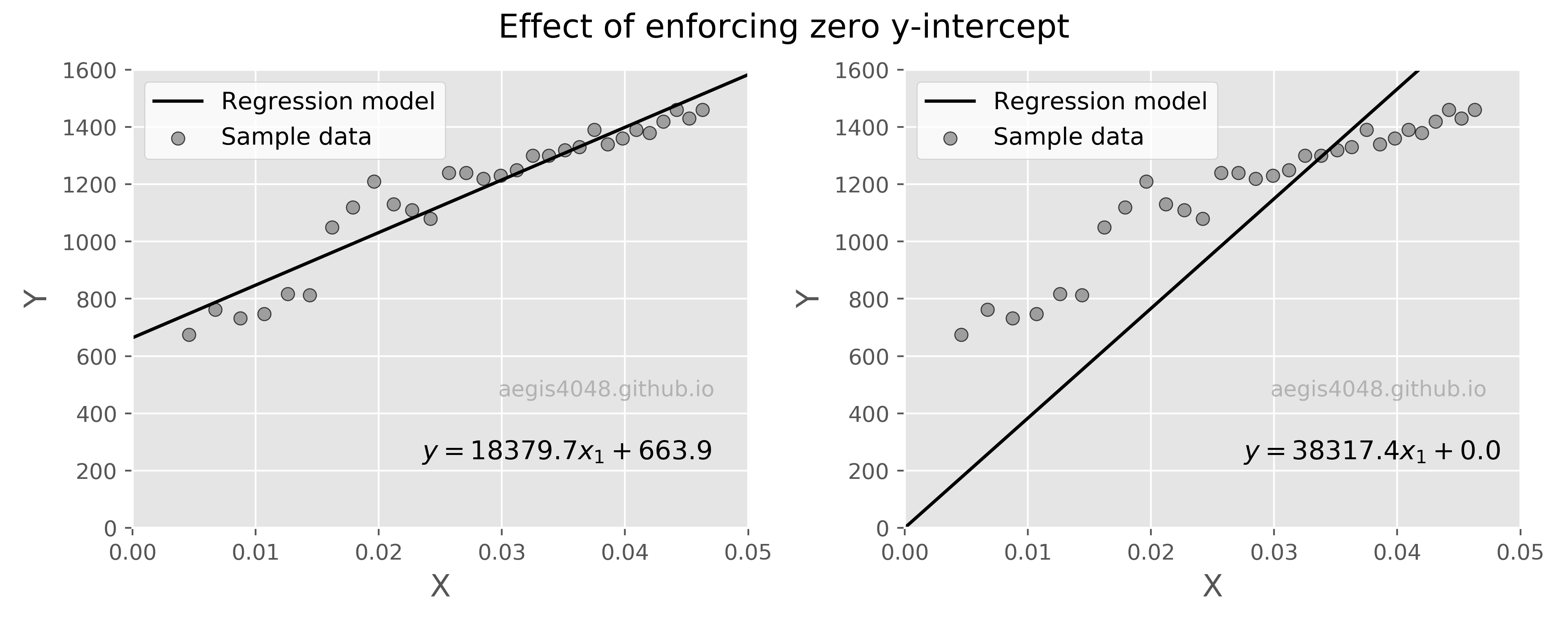
Figure 7: Effect of forcing zero y-intercept
Source Code For Figure (7)
                import pandas as pd
                import numpy as np
                import matplotlib.pyplot as plt
                from sklearn import linear_model

                df = pd.read_csv('https://aegis4048.github.io/downloads/notebooks/sample_data/linear_data.csv')

                features = ['X']
                target = 'Y'

                X = df[features].values.reshape(-1, len(features))
                y = df[target].values

                x_pred = np.linspace(0, 40, 200).reshape(-1, len(features)) # prediction line

                ##################################### Fit linear model ####################################

                ols_1 = linear_model.LinearRegression()
                model_1 = ols_1.fit(X, y)
                response_1 = model_1.predict(x_pred)

                ################################# Force zero y-intercept ##################################

                ols_2 = linear_model.LinearRegression(fit_intercept=False)
                model_2 = ols_2.fit(X, y)
                response_2 = model_2.predict(x_pred)

                ########################################## Plot ###########################################

                plt.style.use('default')
                plt.style.use('ggplot')

                fig, axes = plt.subplots(1, 2, figsize=(10, 4))
                fig.suptitle('Effect of enforcing zero y-intercept', fontsize=15)

                axes[0].plot(x_pred, response_1, color='k', label='Regression model')
                axes[0].scatter(X, y, edgecolor='k', facecolor='grey', alpha=0.7, label='Sample data')
                axes[0].set_ylabel('Y', fontsize=14)
                axes[0].set_xlabel('X', fontsize=14)
                axes[0].legend(facecolor='white', fontsize=11, loc='best')
                axes[0].set_ylim(0, 1600)
                axes[0].set_xlim(0, 0.05)
                axes[0].text(0.47, 0.15, '$y = %.1f x_1 + %.1f $' % (model_1.coef_[0], model_1.intercept_),
                             fontsize=12, transform=axes[0].transAxes)
                axes[0].text(0.77, 0.3, 'aegis4048.github.io', fontsize=10, ha='center', va='center',
                         transform=axes[0].transAxes, color='grey', alpha=0.5)

                axes[1].plot(x_pred, response_2, color='k', label='Regression model')
                axes[1].scatter(X, y, edgecolor='k', facecolor='grey', alpha=0.7, label='Sample data')
                axes[1].set_ylabel('Y', fontsize=14)
                axes[1].set_xlabel('X', fontsize=14)
                axes[1].legend(facecolor='white', fontsize=11, loc='best')
                axes[1].set_ylim(0, 1600)
                axes[1].set_xlim(0, 0.05)
                axes[1].text(0.55, 0.15, '$y = %.1f x_1 + %.1f $' % (model_2.coef_[0], model_2.intercept_),
                             fontsize=12, transform=axes[1].transAxes)
                axes[1].text(0.77, 0.3, 'aegis4048.github.io', fontsize=10, ha='center', va='center',
                         transform=axes[1].transAxes, color='grey', alpha=0.5)

                fig.tight_layout(rect=[0, 0, 1, 0.94])
Pythonic Tip: 3D+ linear regression with scikit-learn
Fit multi-linear model
Let's fit the model with four features: Por, Brittle, Perm, and TOC. Then the model of our interest has the following structure:With scikit-learn, fitting 3D+ linear regression is no different from 2D linear regression, other than declaring multiple features in the beginning. The rest is exactly the same. We will declare four features: features = ['Por', 'Brittle', 'Perm', 'TOC'].
import pandas as pd
import numpy as np
from sklearn import linear_model

file = 'https://aegis4048.github.io/downloads/notebooks/sample_data/unconv_MV_v5.csv'
df = pd.read_csv(file)

features = ['Por', 'Brittle', 'Perm', 'TOC']
target = 'Prod'

X = df[features].values.reshape(-1, len(features))
y = df[target].values

ols = linear_model.LinearRegression()
model = ols.fit(X, y)
model.coef_
model.intercept_
Based on the result of the fit, we obtain the following linear regression model:
Accuracy assessment: $R^2$
In the same we evaluated model performance with 2D linear model above, we can evaluate the 3D+ model performance with R-squared with model.score(X, y). X is the features, and y is the response variable used to fit the model.
model.score(X, y)
Make future prediction
Let's make one prediction of gas production rate when:
- Por = 12 (%)
- Brittle = 81 (%)
- VR = 2.31 (%)
- AI = 2.8 (kg/m2s*10^6)
x_pred = np.array([12, 81, 2.31, 2.8])
x_pred = x_pred.reshape(-1, len(features))
model.predict(x_pred)
This time, let's make two predictions of gas production rate when:
- Por = 12 (%)
- Brittle = 81 (%)
- VR = 2.31 (%)
- AI = 2.8 (kg/m2s*10^6)
- Por = 15 (%)
- Brittle = 60 (%)
- VR = 2.5 (%)
- AI = 1 (kg/m2s*10^6)
x_pred = np.array([[12, 81, 2.31, 2.8], [15, 60, 2.5, 1]])
x_pred = x_pred.reshape(-1, len(features))
model.predict(x_pred)
2. Introduction to multicollinearity
While an accuracy of a multi-linear model in predicting a response variable may be reliable, the value of individual regression coefficient may not be reliable under multicollinearity. Note that the value of regression coefficient for porosity in eq (4) is 287.7, while it is 244.6 in eq (6). In figure (8), I simulated multiple model fits with different combinations of features to show the fluctuating regression coefficient values, even when the R-squared value is high.
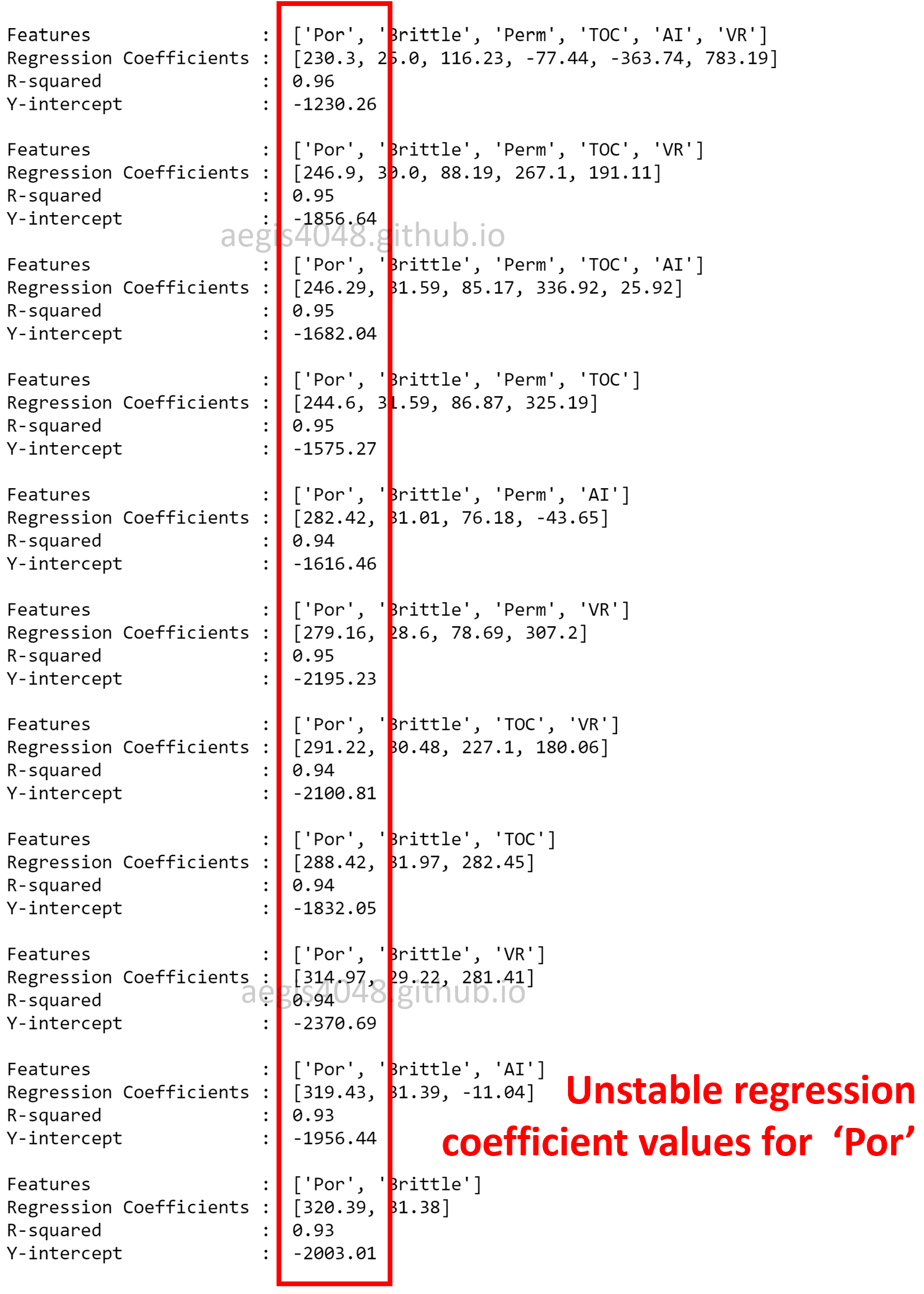
Figure 8: Unstable regression coefficients due to multicollinearity
Source Code For Figure (8)
                import pandas as pd
                import numpy as np
                from sklearn import linear_model
                import matplotlib.pyplot as plt

                file = 'https://aegis4048.github.io/downloads/notebooks/sample_data/unconv_MV_v5.csv'
                df = pd.read_csv(file)

                ########################################################################################

                features = ['Por', 'Brittle', 'Perm', 'TOC', 'AI', 'VR']
                target = 'Prod'

                X = df[features].values.reshape(-1, len(features))
                y = df[target].values

                ols = linear_model.LinearRegression()
                model = ols.fit(X, y)

                print('Features                :  %s' % features)
                print('Regression Coefficients : ', [round(item, 2) for item in model.coef_])
                print('R-squared               :  %.2f' % model.score(X, y))
                print('Y-intercept             :  %.2f' % model.intercept_)
                print('')

                ########################################################################################

                features = ['Por', 'Brittle', 'Perm', 'TOC', 'VR']
                target = 'Prod'

                X = df[features].values.reshape(-1, len(features))
                y = df[target].values

                ols = linear_model.LinearRegression()
                model = ols.fit(X, y)

                print('Features                :  %s' % features)
                print('Regression Coefficients : ', [round(item, 2) for item in model.coef_])
                print('R-squared               :  %.2f' % model.score(X, y))
                print('Y-intercept             :  %.2f' % model.intercept_)
                print('')

                ########################################################################################

                features = ['Por', 'Brittle', 'Perm', 'TOC', 'AI']
                target = 'Prod'

                X = df[features].values.reshape(-1, len(features))
                y = df[target].values

                ols = linear_model.LinearRegression()
                model = ols.fit(X, y)

                print('Features                :  %s' % features)
                print('Regression Coefficients : ', [round(item, 2) for item in model.coef_])
                print('R-squared               :  %.2f' % model.score(X, y))
                print('Y-intercept             :  %.2f' % model.intercept_)
                print('')

                ########################################################################################

                features = ['Por', 'Brittle', 'Perm', 'TOC']
                target = 'Prod'

                X = df[features].values.reshape(-1, len(features))
                y = df[target].values

                ols = linear_model.LinearRegression()
                model = ols.fit(X, y)

                print('Features                :  %s' % features)
                print('Regression Coefficients : ', [round(item, 2) for item in model.coef_])
                print('R-squared               :  %.2f' % model.score(X, y))
                print('Y-intercept             :  %.2f' % model.intercept_)
                print('')

                ########################################################################################

                features = ['Por', 'Brittle', 'Perm', 'AI']
                target = 'Prod'

                X = df[features].values.reshape(-1, len(features))
                y = df[target].values

                ols = linear_model.LinearRegression()
                model = ols.fit(X, y)

                print('Features                :  %s' % features)
                print('Regression Coefficients : ', [round(item, 2) for item in model.coef_])
                print('R-squared               :  %.2f' % model.score(X, y))
                print('Y-intercept             :  %.2f' % model.intercept_)
                print('')

                ########################################################################################

                features = ['Por', 'Brittle', 'Perm', 'VR']
                target = 'Prod'

                X = df[features].values.reshape(-1, len(features))
                y = df[target].values

                ols = linear_model.LinearRegression()
                model = ols.fit(X, y)

                print('Features                :  %s' % features)
                print('Regression Coefficients : ', [round(item, 2) for item in model.coef_])
                print('R-squared               :  %.2f' % model.score(X, y))
                print('Y-intercept             :  %.2f' % model.intercept_)
                print('')

                ########################################################################################

                features = ['Por', 'Brittle', 'TOC', 'VR']
                target = 'Prod'

                X = df[features].values.reshape(-1, len(features))
                y = df[target].values

                ols = linear_model.LinearRegression()
                model = ols.fit(X, y)

                print('Features                :  %s' % features)
                print('Regression Coefficients : ', [round(item, 2) for item in model.coef_])
                print('R-squared               :  %.2f' % model.score(X, y))
                print('Y-intercept             :  %.2f' % model.intercept_)
                print('')

                ########################################################################################

                features = ['Por', 'Brittle', 'TOC']
                target = 'Prod'

                X = df[features].values.reshape(-1, len(features))
                y = df[target].values

                ols = linear_model.LinearRegression()
                model = ols.fit(X, y)

                print('Features                :  %s' % features)
                print('Regression Coefficients : ', [round(item, 2) for item in model.coef_])
                print('R-squared               :  %.2f' % model.score(X, y))
                print('Y-intercept             :  %.2f' % model.intercept_)
                print('')

                ########################################################################################

                features = ['Por', 'Brittle', 'VR']
                target = 'Prod'

                X = df[features].values.reshape(-1, len(features))
                y = df[target].values

                ols = linear_model.LinearRegression()
                model = ols.fit(X, y)

                print('Features                :  %s' % features)
                print('Regression Coefficients : ', [round(item, 2) for item in model.coef_])
                print('R-squared               :  %.2f' % model.score(X, y))
                print('Y-intercept             :  %.2f' % model.intercept_)
                print('')

                ########################################################################################

                features = ['Por', 'Brittle', 'AI']
                target = 'Prod'

                X = df[features].values.reshape(-1, len(features))
                y = df[target].values

                ols = linear_model.LinearRegression()
                model = ols.fit(X, y)

                print('Features                :  %s' % features)
                print('Regression Coefficients : ', [round(item, 2) for item in model.coef_])
                print('R-squared               :  %.2f' % model.score(X, y))
                print('Y-intercept             :  %.2f' % model.intercept_)
                print('')

                ########################################################################################

                features = ['Por', 'Brittle']
                target = 'Prod'

                X = df[features].values.reshape(-1, len(features))
                y = df[target].values

                ols = linear_model.LinearRegression()
                model = ols.fit(X, y)

                print('Features                :  %s' % features)
                print('Regression Coefficients : ', [round(item, 2) for item in model.coef_])
                print('R-squared               :  %.2f' % model.score(X, y))
                print('Y-intercept             :  %.2f' % model.intercept_)
The simulation result tells us that even if the model is good at predicting the response variable given features (high R-squared), linear model is not robust enough to fully understand the effect of individual features on the response variable. In such circumstance, we can't trust the values of regression coefficients. Where is this instability coming from? This is because the Por, TOC, and Perm shows strong linear correlation with one another, as shown in the below spearnman's correlation matrix in figure (9).
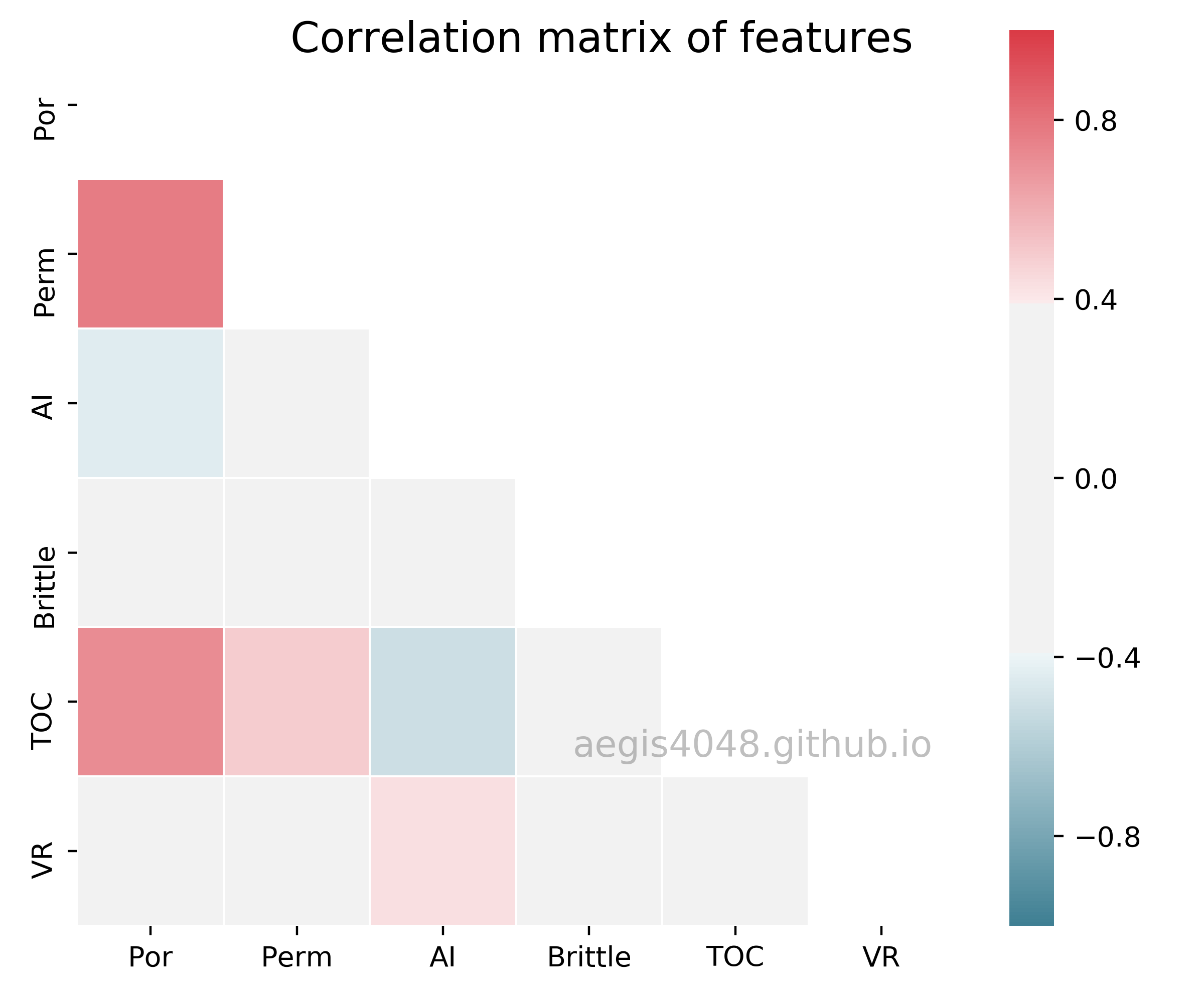
Figure 9: Correlation matrix of features
Source Code For Figure (9)
                import numpy as np
                import pandas as pd
                import seaborn as sns
                import matplotlib.pyplot as plt

                file = 'https://aegis4048.github.io/downloads/notebooks/sample_data/unconv_MV_v5.csv'
                df = pd.read_csv(file)

                df = df.iloc[:, 1:-1]

                corr = df.corr(method='spearman')

                # Generate a mask for the upper triangle
                mask = np.zeros_like(corr, dtype=np.bool)
                mask[np.triu_indices_from(mask)] = True

                # Set up the matplotlib figure
                fig, ax = plt.subplots(figsize=(6, 5))

                # Generate a custom diverging colormap
                cmap = sns.diverging_palette(220, 10, as_cmap=True, sep=100)

                # Draw the heatmap with the mask and correct aspect ratio
                sns.heatmap(corr, mask=mask, cmap=cmap, vmin=-1, vmax=1, center=0, linewidths=.5)

                fig.suptitle('Correlation matrix of features', fontsize=15)
                ax.text(0.77, 0.2, 'aegis4048.github.io', fontsize=13, ha='center', va='center',
                         transform=ax.transAxes, color='grey', alpha=0.5)

                fig.tight_layout()
When more than two features are used for prediction, you must consider the possibility of each features interacting with one another. For thought experiment, think of two features $x_1$ and $x_2$, and a response variable $y$. Assume that $x_1$ is positively related to $y$. In the other words, increasing $x_1$ increases $y$, and decreasing $x_1$ also decreases $y$. $x_2$ is negatively related to $y$. There is a positive correlation between $x_1$ and $x_2$. Under this sitution, when you increase $x_1$, you expect to increase the value of $y$ because of the positive relationship between $x_1$ and $y$, but this is not always true because increasing $x_1$ also increases $x_2$, which in turn decreases $y$ .
The situation in which features are correlated with one another is called muticollinearity. Under multicollinearity, the values of individual regression coefficients are unreliable, and the impact of individual features on a response variable is obfuscated. However, prediction on a response variable is still reliable.
When using linear regression coefficients to make business decisions, you must remove the effect of multicollinearity to obtain reliable regression coefficients. Let's say that you are doing a medical research on cervical cancer. You trained a linear regression model with patients' survival rate with respect to many features, in which water consumption being one of them. Your linear regression coefficient for water consumption reports that if a patient increases water consumption by 1.5 L everyday, his survival rate will increase by 2%. Can you trust this analysis? The answer is yes, if there is no sign of multicollinearity. You can actually tell the patient, with confidence, that he must drink more water to increase his chance of survival. However, if there is a sign of multicollinearity, this analysis is not valid.
Note that multicollinearity is not restricted on 1 vs 1 relationship. Even if there is minimum 1 vs 1 correlation among features, three or more features together may show multicollinearity. Also note that multicollinearity does not affect prediction accuracy. While the values of individual coefficients may be unreliable, it does not undermine the prediction power of the model. Multicollinearity is an issue only when you want to study the impact of individual features on a response variable.
The details of detection & remedies of mutlicollinearity is not discussed here (though I plan to write about it very soon). While the focus of this post is only on multiple linear regression itself, I still wanted to grab your attention as to why you should not always trust your regression coefficients.
Related Posts
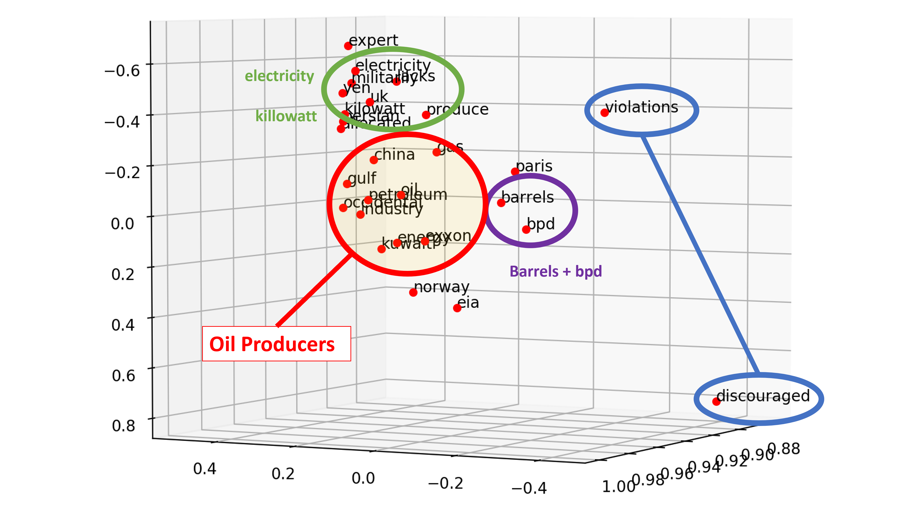
Understanding Multi-Dimensionality in Vector Space Modeling
How does word vectors in Natural Language Processing capture meaningful relationships among words? How can you quantify those relationships? Addressing these questions starts from understanding the multi-dimensional nature of NLP applications.
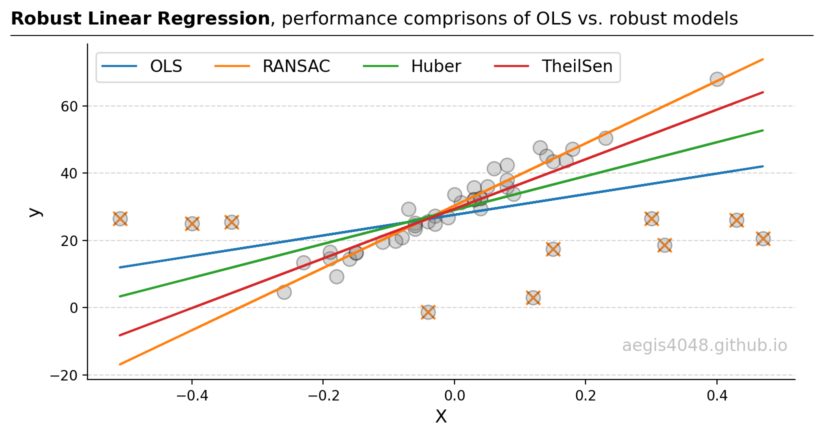
Robust Linear Regressions In Python
In regression, managing outliers is key for accurate predictions. Techniques like OLS can be skewed by outliers. This analysis compares OLS, RANSAC, Huber, and Theil-Sen methods, showing how each deals with outliers differently, using theory and Python examples, to guide the best model choice for different outlier scenarios.