Non-Parametric Confidence Interval with Bootstrap
Category > Statistics
Jan 04, 2019The code snippet assumes Anaconda 5.2.0 version of Python virtual environment
Acknowledgement
I would like to acknowledge Micahel Pyrcz, Associate Professor at the University of Texas at Austin in the Petroleum and Geosystems Engineering, for developing course materials that helped me write this article.
Check out his Youtube Lecture on Bootstrap, and Boostrap Excel numerical demo on his Github repo to help yourself better understand the statistical theories and concepts.
Bootstrap is a non-parametric statistical technique to resample from known samples to estimate uncertainty in summary statistics. When there are small, limited number of samples, it gives a more accurate forecast model than directly obtaining a forecast model from the limited sample pool (assuming that the sample set of data is reasonable representation of the population). It is non-parametric because it does not require any prior knowledge of the distribution (shape, mean, standard devation, etc..).
Advantages of Bootstrap
One great thing about Bootstrapping is that it is distribution-free. You do not need to know distribution shape, mean, standard devation, skewness, kurtosis, etc... All you need is just a set of sample data that is representative of a population. The fact that Bootstrapping does not depend on a type of distribution leads to another great advantage - It can calculate uncertainty in any confidence interval of any kind of distribution.
For example, the analytical solution to calculate a confidence interval in any statistics of a distribution is as follows:
There are three problems with analytically solving for confidence interval of a statistic.
First, the variable in the equation, distribution score, depends on the type of the distribution. If you do not know the distribution shape of your population, it is very difficult to calculate the confidence interval of a statistic.
Second, not all statistics have a formula to calculate its Standard Error. For example, there exists an equation to calculate the standard error of a mean:
But there is no equation to calculate the standard error of a median. If you want to obtain confidence intervals for other statistics (ex: skewness, kurtosis, IQR, etc...), it will be very difficult to do so, simply because there are no equations for them.
Third, some statistics have analytical solutions for its standard error calculation, but it is so convoluted that Bootstrapping is simpler. A classic example is obtaining a CI for the correlation coefficient given a sample from a bivariate normal distribution.
Bootstrapping calculates confidence intervals for summary statistics numerically, not analytically, and this is why it can calculate ANY summary stats for ANY distribution.
Methodology
One goal of inferential statistics is to determine the value of a parameter of an entire population. It is typically too expensive or even impossible to measure this directly. So we use statistical sampling. We sample a population, measure a statistic of this sample, and then use this statistic to say something about the corresponding parameter of the population.
Bootstrapping is a type of resampling method to save time and money taking measurements. From a sample pool of size N, it picks a random value N times with replacement, and create M number of new Bootstrapped-sample pools. The term with replacement here means that you put back the sample you drew to the original sample pool after adding it to a new Bootstrapped-sample pool. Think of it this way: you randomly choose a file from a folder in your PC, and you copy and paste the randomly-chosen file into a new folder. You do not cut and paste the file, but you copy and paste the file into a new folder. You will have M number of folders (M is an arbitrary number of your choice), each containing N number of files.
Bootstrapping resamples the original sample pool to generate multiple smaller population of the true population. Each Bootstrap simulation is done by selecting a random value from the sample pool. For example, lets assume that you have the following sample pool of integers:
From the sample pool of size N=7, you choose a random value N=7 times, and create a new sample pool of size N=7. In Bootstrap, each newly created sample pool is called a realization. You generate many of these realizations, and use them to calculate uncertainties in summary stats.
Notice the duplicate data in the realizations (Ex: 533, 533, 533). Duplicates in realizations exist because each data in realization is randomly chosen from the original sample pool with replacement.
Warning!
It is extremly important that the N size for each Bootstrap realization matches the N size of the original sample pool.
We use Bootstrap to numerically estimate the confidence interval (CI). It's an alternative tool to analytically solve for CI. Observing how CI is analytically calculated may help one to understand why the value of N is important. Let's take the CI of a mean for example. Recall that the CI of a mean represents how far a sample mean can deviate from the true population mean.
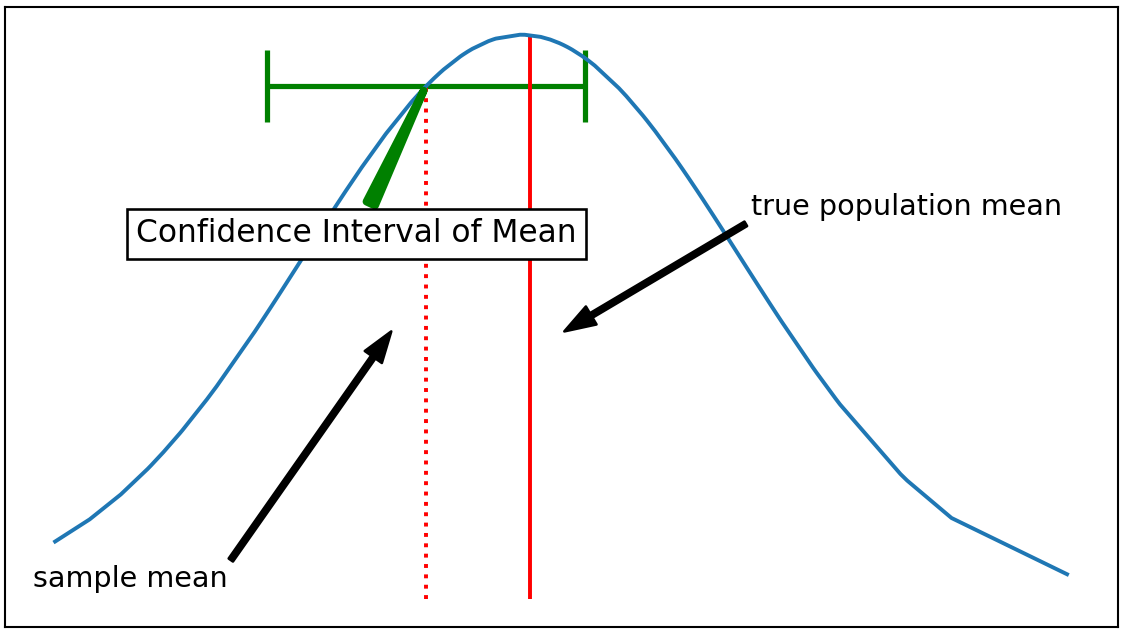
In case of a Gaussian, or Gaussian-like distribution (ex: student-t), the equation to analytically solve for confidence interval of a mean is as follows:
The size of each Bootstrap realization, N, works the similar way, except that the random sample in each realization is not from the true population, but from a measured sample pool. Increasing the N-value will falsely make you to calculate smaller confidence interval.
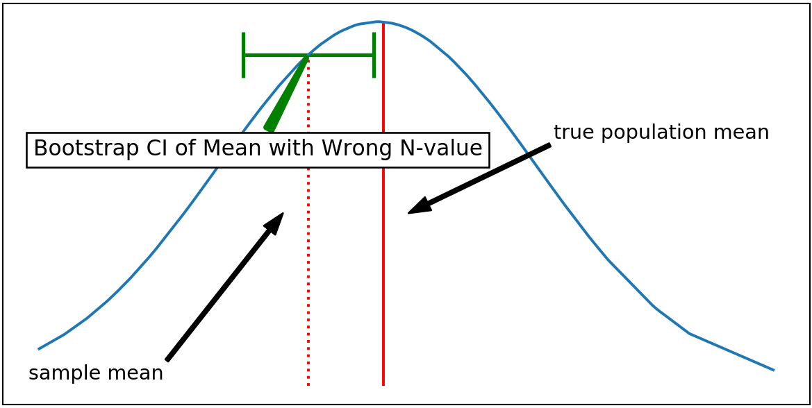
It can be observed that the CI obtained by using a wrong N-value for Bootstrap generates narrower CI. As a result, the CI of the sample mean does not cover the true population mean, returning a misleading estimation.
In summary, Bootstrapping is used for three reasons:
- Bootstrap can obtain confidence interval in any statistics.
- Bootstrap does not assume anything about a distribution.
- Bootstrap helps when there are too few number of samples.
Imports
import pandas as pd
import numpy as np
import scipy.stats
import matplotlib.pyplot as plt
import matplotlib.gridspec as gridspec
%matplotlib notebook
1.A. Confidence Intervals in Summary Stats: US Male Height - Gaussian Distribution
Bootstrap simulation can be run to obtain confidence intervals in various population parameters: mean, stdev, variance, min, or max. In this example, we will work with the height distribution of the US Male population, which tends to be Gaussian. However, the fact that the distribution Gaussian is totally unrelated to Bootstrap simulation, because it does not assume anything about the distribution.
Bootstrapping can give us confidence intervals in any summary statistics like the following:
By 95% chance, the following statistics will fall within the range of:
Mean : 75.2 ~ 86.2, with 80.0 being the average
Standard Deviation : 2.3 ~ 3.4 with 2.9 being the average
Min : 54.3 ~ 57.2, with 55.2 being the average
Max : 77.8 ~ 82.4, with 79.8 being the average
Skew : -0.053 ~ 0.323, with 0.023 being the average
1.A.0. Bootstrap Scripts
Bootstrap Simulator
def bootstrap_simulation(sample_data, num_realizations):
    n = sample_data.shape[0]
    boot = []
    for i in range(num_realizations):
        real = np.random.choice(sample_data.values.flatten(), size=n)
        boot.append(real)

    columns = ['Real ' + str(i + 1) for i in range(num_realizations)]

    return pd.DataFrame(boot, index=columns).T
Summary Statistics Calculator
def calc_sum_stats(boot_df):
    sum_stats = boot_df.describe().T[['mean', 'std', 'min', 'max']]
    sum_stats['median'] = boot_df.median()
    sum_stats['skew'] = boot_df.skew()
    sum_stats['kurtosis'] = boot_df.kurtosis()
    sum_stats['IQR'] = boot_df.quantile(0.75) - boot_df.quantile(0.25)
    return sum_stats.T
Visualization Script
def visualize_distribution(dataframe, ax_):
    dataframe = dataframe.apply(lambda x: x.sort_values().values)

    for col, label in zip(dataframe, dataframe.columns):
        fit = scipy.stats.norm.pdf(dataframe[col], np.mean(dataframe[col]), np.std(dataframe[col]))
        ax_.plot(dataframe[col], fit)
    ax_.set_ylabel('Probability')
Generate Confidence Intervals
def calc_bounds(conf_level):

    assert (conf_level < 1), "Confidence level must be smaller than 1"

    margin = (1 - conf_level) / 2
    upper = conf_level + margin
    lower = margin
    return margin, upper, lower

def calc_confidence_interval(df_sum_stats, conf_level):

    margin, upper, lower = calc_bounds(conf_level)

    conf_int_df = df_sum_stats.T.describe(percentiles=[lower, 0.5, upper]).iloc[4:7, :].T
    conf_int_df.columns = ['P' + str(round(lower * 100, 1)), 'P50', 'P' + str(round(upper * 100, 1))]
    return conf_int_df

def print_confidence_interval(conf_df, conf_level):
    print('By {}% chance, the following statistics will fall within the range of:\n'.format(round(conf_level * 100, 1)))

    margin, upper, lower = calc_bounds(conf_level)

    upper_str = 'P' + str(round(upper * 100, 1))
    lower_str = 'P' + str(round(lower * 100, 1))

    for stat in conf_df.T.columns:
        lower_bound = round(conf_df[lower_str].T[stat], 1)
        upper_bound = round(conf_df[upper_str].T[stat], 1)

        mean = round(conf_df['P50'].T[stat], 1)
        print("{0:<10}: {1:>10}  ~ {2:>10} , AVG = {3:>5}".format(stat, lower_bound, upper_bound, mean))
1.A.1 Sample Data Description
100 samples of US male height data is provided in my Github Repo - sample_data/US_Male_Height.csv. Summary statistics of the sample data can be calculated. Your goal is to calculate the confidence intervals for the summary stats.
# height data

height_data = pd.read_csv('sample_data/US_Male_Height.csv')
height_data.index = ['Male ' + str(i + 1) for i in range(height_data.shape[0])]
height_data.round(1).T
height_summary_stats = calc_sum_stats(height_data)
height_summary_stats
Visualization
fig, ax = plt.subplots(figsize=(8, 4))
ax.set_xlabel('Height (inches)');
fig.suptitle('Original Sample Data Distribution: Gaussian Distribution')

visualize_distribution(height_data, ax);

Based on the distribution plot of the original sample data, we can observe that the distribution indeed looks Gaussian. However, the fact that it looks like Gaussian does not matter at all when Bootstrapping, because Bootstrapping does not assume anything about the distribution.
1.A.2 Resampling From the Sample Data
Each Bootstrap resampling (realization) can be done in one-line with numpy.random.choice(). Each realization is an array of size N, where N is the length of the original sample data. There are M number of realizations, where M is an arbitrary number of your choice.
Results
M = 100                                                 # number of realizations - arbitrary
bootstrap_data = bootstrap_simulation(height_data, M)
bootstrap_data.round(1).head(10)
boot_sum_stats = calc_sum_stats(bootstrap_data)
boot_sum_stats.round(1)
Visualize
fig, ax = plt.subplots(figsize=(8, 4))
ax.set_xlabel('Height (inches)');
fig.suptitle('Distribution of Bootstrap-Simulated Data: Gaussian')
visualize_distribution(bootstrap_data, ax);

Each line in the plot represents one Bootstrap realization. There are 100 realizations, each having 100 random samples.
1.A.3 Uncertainty Models in Summary Statistics with Blox Plots
f = plt.figure()
plt.suptitle('Uncertainty Models for Various Statistics: US Male Height - Gaussian')

gs = gridspec.GridSpec(2, 4)
ax1 = plt.subplot(gs[0, 0:4])
ax2 = plt.subplot(gs[1, 0])
ax3 = plt.subplot(gs[1, 1])
ax4 = plt.subplot(gs[1, 2])
ax5 = plt.subplot(gs[1, 3])

boot_sum_stats.T[['mean', 'min', 'max', 'median']].boxplot(ax=ax1)
boot_sum_stats.T[['std']].boxplot(ax=ax2)
boot_sum_stats.T[['IQR']].boxplot(ax=ax3)
boot_sum_stats.T[['skew']].boxplot(ax=ax4)
boot_sum_stats.T[['kurtosis']].boxplot(ax=ax5)

ax5.set_ylim([-3, 3]);

1.A.4 Confidence Interval in Summary Statistics
Confidence intervals of summary statistics usually have a confidence level of 90%, 95%, or 99%. In this case, we will choose 95% confidence level.
confidence_level = 0.95

conf_int = calc_confidence_interval(boot_sum_stats, confidence_level)
conf_int.round(1)
print_confidence_interval(conf_int, confidence_level)
1.B. Confidence Intervals in Summary Stats: Rock Permeability - Lognormal Distribution
It was previously stated that Bootstrapping does not assume anything about the distribution. Is that really true? The previous example of the US Male Height distribution was a Gaussian distribution. But what if the distribution of our interest is not Gaussian?
In this example, rock pearmeability, which has a lognormal distribution, will be used to show that Bootstrap does not depend on the type of the distribution.
1.B.0. Bootstrap Scripts
The sample scripts used for US Male Height example will be used for Bootstrap simulation. Same scripts can be used for both Gaussian and lognormal distribution because Bootstrapping does not assume anything about the distribution.
1.B.1. Sample Data Description
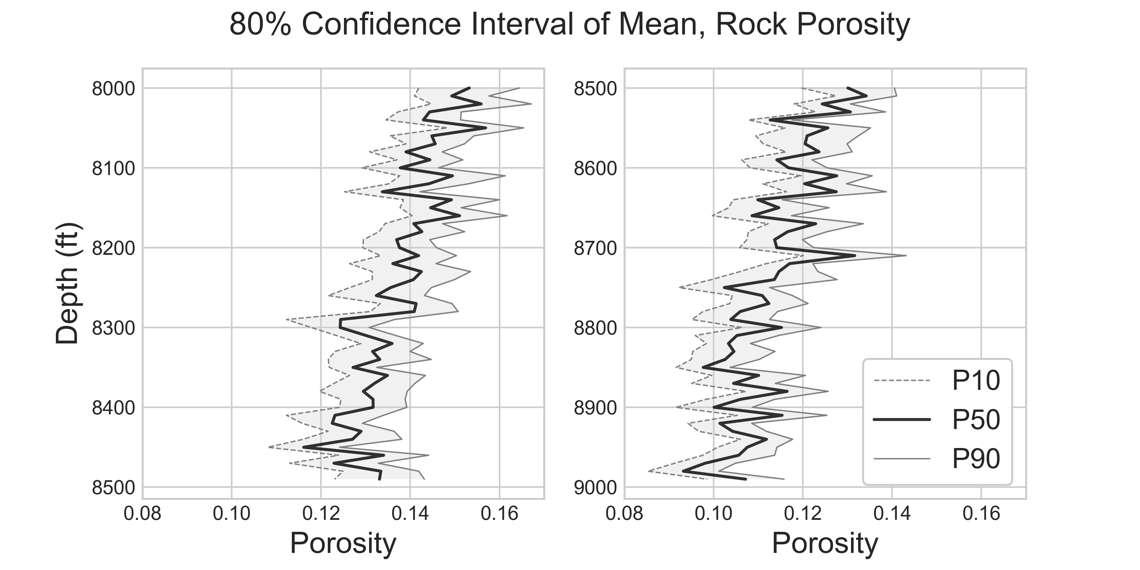
105 samples of permeability data is provided in Github Repo - sample_data/PoroPermSampleData.xlsx. Permeability data is taken at many times at different depth of a wellbore.
Summary statistics of the sample data can be calculated. Your goal is to calculate the confidence intervals for the summary stats.
# permeability data
perm_depth_data = pd.read_excel('sample_data/PoroPermSampleData.xlsx', sheet_name='Sheet1')[['Depth', 'Permeability (mD)']]
perm_data = perm_depth_data['Permeability (mD)'].to_frame()

# visualize
fig = plt.figure()
ax = plt.axes()

ax.plot(perm_depth_data['Permeability (mD)'], perm_depth_data['Depth']);
ax.invert_yaxis()
ax.set_title('Permeability Along A Wellbore')
ax.set_xlabel('Permeability (mD)')
ax.set_ylabel('Depth (ft)');

perm_summary_stats = calc_sum_stats(perm_data)
perm_summary_stats
Visualization
fig, ax = plt.subplots(figsize=(8, 4))
ax.set_xlabel('Permeability (mD)')
fig.suptitle('Original Sample Data Distribution: Lognormal Distribution')
visualize_distribution(perm_data, ax);

Based on the distribution of the original sample data, we can observe that the distribution looks lognormal. The uncertainty in summary statistics can be calculated using Bootstrap the same way it was done for the US Male Height (Gaussian) distribution, because Bootstrap does not depend on the shape of the distribution.
Warning!
Outlier removal on rock permeability cannot be done directly, as this is a lognormal distribution. Recall that the typical outlier removal method assumes the distribution to be Gaussian. If you want to detect outliers for non-Gaussian distributions, you have to first transform the distribution into Gaussian.
1.B.2 Resampling From the Sample Data
Each Bootstrap resampling (realization) can be done in one-line with numpy.random.choice(). Each realization is an array of size N, where N is the length of the original sample data. There are M number of realizations, where M is an arbitrary number of your choice.
Results
M = 100                      # number of realizations - arbitrary
boot_perm_data = bootstrap_simulation(perm_data, M)
boot_perm_data.round(1).head(10)
boot_perm_sum_stats = calc_sum_stats(boot_perm_data)
boot_perm_sum_stats.round(1)
Visualize
fig, ax = plt.subplots(figsize=(8, 4))
fig.suptitle('Distribution of Bootstrap-Simulated Data: Lognormal')
ax.set_xlabel('Permeability (mD)')
visualize_distribution(boot_perm_data, ax);

1.B.3 Uncertainty Models in Summary Statistics with Blox Plots
f = plt.figure()
plt.suptitle('Uncertainty Models for Various Statistics: Rock Permeability - Lognormal')

gs = gridspec.GridSpec(2, 4)
ax1 = plt.subplot(gs[0, 0:4])
ax2 = plt.subplot(gs[1, 0])
ax3 = plt.subplot(gs[1, 1])
ax4 = plt.subplot(gs[1, 2])
ax5 = plt.subplot(gs[1, 3])

boot_perm_sum_stats.T[['mean', 'min', 'max', 'median']].boxplot(ax=ax1)
boot_perm_sum_stats.T[['std']].boxplot(ax=ax2)
boot_perm_sum_stats.T[['IQR']].boxplot(ax=ax3)
boot_perm_sum_stats.T[['skew']].boxplot(ax=ax4)
boot_perm_sum_stats.T[['kurtosis']].boxplot(ax=ax5)

ax4.set_ylim([-3, 3])
ax5.set_ylim([-10, 10]);

Observe the positive skewness in the boxplot summary statistics. This is consistent with the left-justified lognormal distribution of the permeability plot.
1.B.4 Confidence Interval in Summary Statistics
Confidence intervals of summary statistics usually have a confidence level of 90%, 95%, or 99%. In this case, we will choose 90% confidence level.
confidence_level = 0.9

conf_int_perm = calc_confidence_interval(boot_perm_sum_stats, confidence_level)
conf_int_perm.round(1)
print_confidence_interval(conf_int_perm, confidence_level)
Related Posts
Uncertainty Modeling with Monte-Carlo Simulation
How do casinos earn money? The answer is simple - the longer you play, the bigger the chance of you losing the money. Monte-Carlo simulation can construct its profit forecast model.
Transforming Non-Normal Distribution to Normal Distribution
Many statistical & machine learning techniques assume normality of data. What are the options you have if your data is not normally distributed? Transforming non-normal data to normal data using Box-Cox transformation is one of them.
Comprehensive Confidence Intervals for Python Developers
This post covers everything you need to know about confidence intervals: from the introductory conceptual explanations, to the detailed discussions about the variations of different techniques, their assumptions, strength and weekness, when to use, and when not to use.
Robust Linear Regressions In Python
In regression, managing outliers is key for accurate predictions. Techniques like OLS can be skewed by outliers. This analysis compares OLS, RANSAC, Huber, and Theil-Sen methods, showing how each deals with outliers differently, using theory and Python examples, to guide the best model choice for different outlier scenarios.