Demystifying Neural Network in Skip-Gram Language Modeling
Category > Natural Language Processing
May 06, 2019Contents
- 1. Paradigm shift in word embedding: count-based to prediction-based
- 2. Prediction-based word-embedding: Word2Vec Skip-Gram
- Notes:CBOW and Skip-Gram
- 2.1. Why predict context words?
- 2.2. What is the application of vector representations of words?
- 3. Derivation of cost function
- 4. Window size of Skip-Gram
- 5. Neural network structure of Skip-Gram
- 5.1. Training: forward propagation
- 5.1.1. Input layer ($x$)
- 5.1.2. Input and output weight matrix ($W_{input}$,-$W_{output}$)
- 5.1.3. Hidden (projection) layer ($h$)
- 5.1.4. Softmax output layer ($y_{pred}$)
- 5.2. Training: backward propagation
- 6. Numerical demonstration
Acknowledgement
The materials on this post are based the on two NLP papers, Distributed Representations of Words and Phrases and their Compositionality (Mikolov et al., 2013) and word2vec Parameter Learning Explained (Rong, 2014).
1. Paradigm shift in word embedding: count-based to prediction-based
Up until 2013, the traditional models for NLP tasks were count-based models. They mainly involve computing a co-occurence matrix to capture meaningful relationships among words (If you are interested in how co-occurrence matrix is used for language modeling, check out Understanding Multi-Dimensionality in Vector Space Modeling). For example:
Document 1: "all that glitters is not gold"
Document 2: "all is well that ends well"
| * | START | all | that | glitters | is | not | gold | well | ends | END |
|---|---|---|---|---|---|---|---|---|---|---|
| START | 0 | 2 | 0 | 0 | 0 | 0 | 0 | 0 | 0 | 0 |
| all | 2 | 0 | 1 | 0 | 1 | 0 | 0 | 0 | 0 | 0 |
| that | 0 | 1 | 0 | 1 | 0 | 0 | 0 | 1 | 1 | 0 |
| glitters | 0 | 0 | 1 | 0 | 1 | 0 | 0 | 0 | 0 | 0 |
| is | 0 | 1 | 0 | 1 | 0 | 1 | 0 | 1 | 0 | 0 |
| not | 0 | 0 | 0 | 0 | 1 | 0 | 1 | 0 | 0 | 0 |
| gold | 0 | 0 | 0 | 0 | 0 | 1 | 0 | 0 | 0 | 1 |
| well | 0 | 0 | 1 | 0 | 1 | 0 | 0 | 0 | 1 | 1 |
| ends | 0 | 0 | 1 | 0 | 0 | 0 | 0 | 1 | 0 | 0 |
| END | 0 | 0 | 0 | 0 | 0 | 0 | 1 | 1 | 0 | 0 |
Table 1: Co-Occurence Matrix
Count-based language modeling is easy to comprehend — related words are observed (counted) together more often than unrelated words. Many attempts were made to improve the performance of the model to the state-of-art, using SVD, ramped window, and non-negative matrix factorization (Rohde et al. ms., 2005), but the model did not do well in capturing complex relationships among words.
Then, the paradigm started to change in 2013, when Thomas Mikolov proposed the prediction-based modeling technique, called Word2Vec, in his famous paper, Distributed Representations of Words and Phrases and their Compositionality. Unlike counting word co-occurrences, the model uses neural networks to learn intelligent representation of words in a vector space. Then, the paper submitted to ACL in 2014, Don’t count, predict! A systematic comparison of context-counting vs. context-predicting semantic vectors, quantified & compared the performances of count-based vs prediction-based models.
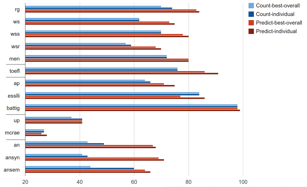
Figure 1: Performance comparison of models (source)
The blue bars represent the count-based models, and the red bars are for prediction-based models. The full summary of the paper and more detailed description about the result graph can be found here. Long story short, prediction-based models outperformed count-based models by a large margin on various language tasks.
2. Prediction-based word-embedding: Word2Vec Skip-Gram
One of the prediction-based language model introduced by Mikolov is Skip-Gram:
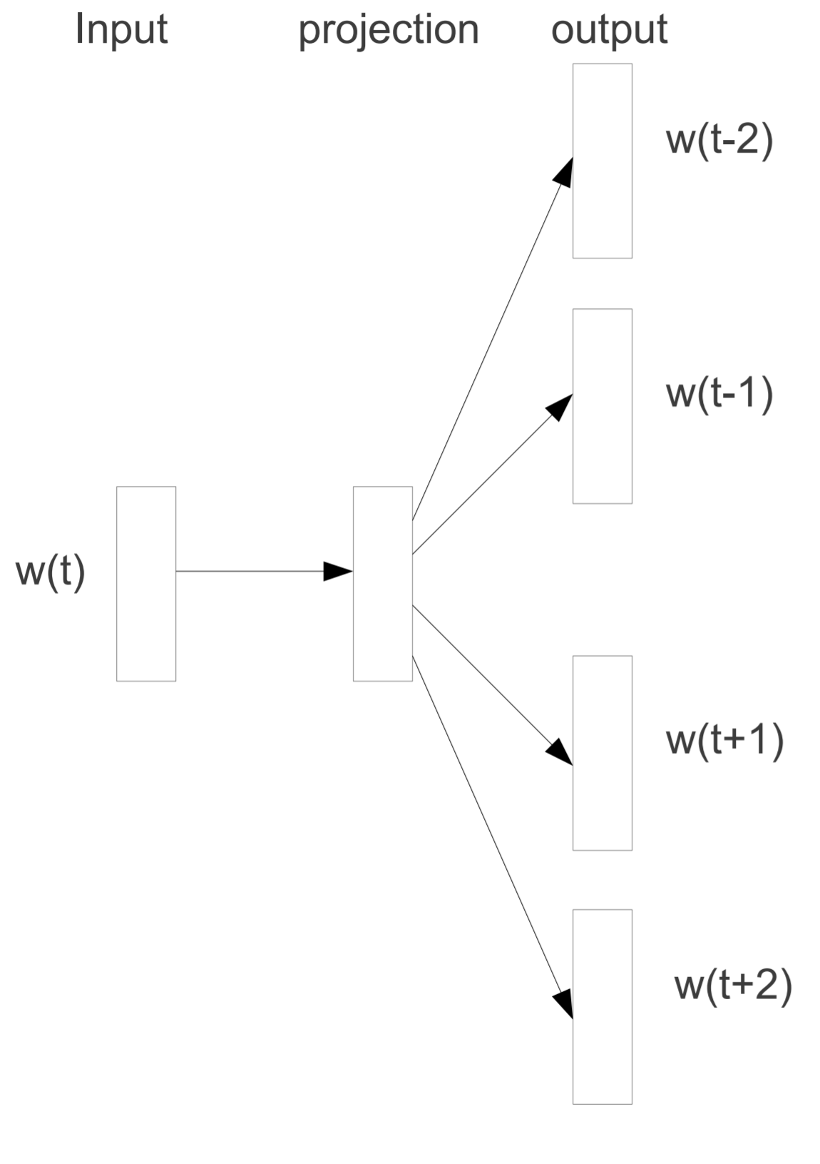
Figure 2: Original Skip-gram model architecture
Figure 2 is a diagram presented in the original Word2Vec paper. It is essentially describing that the model uses a neural network of one hidden (projection) layer to correctly predict context words $w(t-2)$, $w(t-1)$, $w(t+1)$, $w(t+2)$ of an input word $w(t)$. In the other words, the model attempts to maximize the probability of observing all four context words together, given a center word. Mathematically, it can be denoted as eq-1. The training objective is to learn word vector representations that are good at predicting the nearby words.
Notes: CBOW and Skip-Gram
There are two models for Word2Vec: Continous Bag Of Words (CBOW) and Skip-Gram. While Skip-Gram model predicts context words given a center word, CBOW model predicts a center word given context words. According to Mikolov:
Skip-gram: works well with small amount of the training data, represents well even rare words or phrases
CBOW: several times faster to train than the skip-gram, slightly better accuracy for the frequent words
Skip-Gram model is a better choice most of the time due to its ability to predict infrequent words, but this comes at the price of increased computational cost. If training time is a big concern, and you have large enough data to overcome the issue of predicting infrequent words, CBOW model may be a more viable choice. The details of CBOW model won't be covered in this post.
2.1. Why predict context words?
A natural question is, why do we predict context words? One must understand that the ultimate goal of Skip-Gram model is not to predict context words, but to learn intelligent vector representation of words. It just happens that predicting context words inevitably results in good vector representations of words, because of the neural network structure of Skip-Gram. Neural network at its essence is just optimizing weight marices $\theta$ to correctly predict output. In Word2Vec Skip-Gram, the weight matrices are, in fact, the vector representations of words. Therefore, optimizing weight matrix = good vector representations of words. This is described in detail below.
2.2. What is the application of vector representations of words?
In Word2Vec, words are represented as vectors, and related words are placed closed to each other on a vector space. Mathematically, this means that the vector distance between related words are smaller than the vector distance between unrelated words.
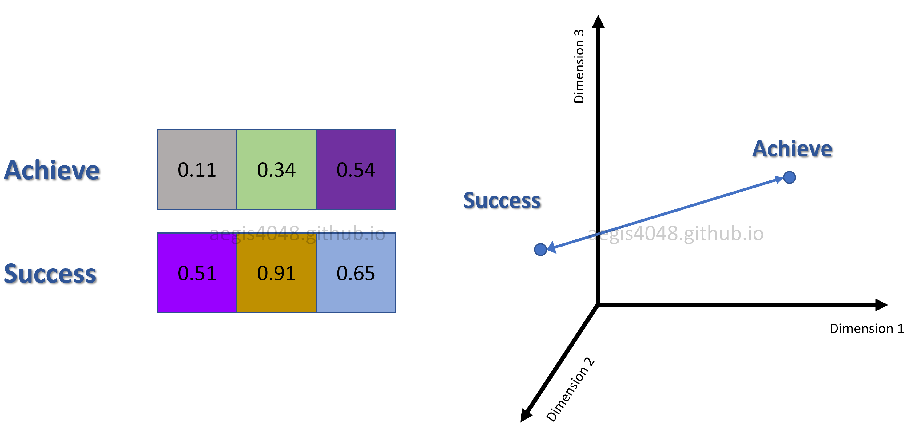
Figure 3: Vector distance between two words
For example in Figure 3, correlation between "success" and "achieve" can be quantified by computing the vector distance between them (Notes: For illustration purpose, three-dimensional word vectors are assumed in the figure, because higher dimensional vectors can't be visualized. Also, distance annotated in the figure is Euclidean, but in real-life, we use Cosine distance to evaluate vector correlations).
One interesting application of vector representaion of words is that it can be used to solve analogy tasks. Let's assume the following word vectors for "Germany", "capital", and "Berlin".
$$ \begin{align*} vec(\text{Germany}) & = [1.22 \quad 0.34 \quad -3.82] \\ vec(\text{capital}) & = [3.02 \quad -0.93 \quad 1.82] \\ vec(\text{Berlin}) & = [4.09 \quad -0.58 \quad 2.01] \end{align*} $$To find out the capital of Germany, the word vector of "capital" can be added to the word vector of "Germany".
$$ \begin{align*} vec(\text{Germany}) + vec(\text{capital}) &= [1.22 \quad 0.34 \quad -3.82] + [3.02 \quad -0.93 \quad 1.82] \\ &= [4.24 \quad -0.59 \quad -2.00] \end{align*} $$Since the sum of the word vectors of "Germany" and "capital" is similar to the word vector of "Berlin", the model may conclude that the capital of Germany is Berlin.
$$ \begin{align*} [4.24 \quad -0.59 \quad -2.00] & \cong [4.09 \quad -0.58 \quad 2.01] \\ vec(\text{Germany}) + vec(\text{capital}) & \cong vec(\text{Berlin}) \end{align*} $$Notes: Analogy tasks don't always work
Not all analogy tasks can be solved like this. The above illustration works like a magic, but there are many analogy problems that can't be solved with Word2Vec. Think of the above illustration as just one use case of Word2Vec.
3. Derivation of cost function
Skip-Gram model seeks to optimize the word weight (embedding) matrix by correctly predicting context words, given a center word. In the other words, the model wants to maximize the probability of correctly predicting all context words at the same time, given a center word. Maximizing the probability of predicting context words leads to optimizing the weight matrix ($\theta$) that best represents words in a vector space. $\theta$ is a concatenation of input and output weight matrices — $[W_{input} \quad W_{output}]$, as described below. It is passed into the cost function ($J$) as a variable and optimized. Mathematically, it can be expressed as:
where $C$ is the window size, and $w$ is a word vector (which can be a context or a center word). Recall that in statistics, the probability of $A$ given $B$ is expressed as $P(A|B)$. Then, natural log is taken on eq-1 to simplify taking derivatives.
Notes: Why take a natural log?
In machine learning, it is a common practice to take a natural log to the objective function to simplify taking derivatives. For example, a multinomial regression classifer called Softmax (details explained below) has the following probability function:
Taking a log simplifies the function:
Depending on a model, the argument ($x_i$) passed into the probability function ($p$) can be complicated, and simplifying the original softmax function helps with taking the derivatives in the future.
Taking a log does not affect the optimized weights ($\theta$), because natural log is a monotonically increasing function. This means that increasing the value of $x$-axis results in increasing the value of $y$-axis. This is important because it ensures that the maximum value of the original probability function occurs at the same point as the log probability function. Therefore:
In Skip-Gram, softmax function is used for context words classfication. The details are explained below. Softmax in Skip-Gram has the following equation:
$W_{output_{(context)}}$ is a row vector for a context word from the output embedding matrix (see below), and $h$ is the hidden (projection) layer word vector for a center word (see below). Softmax function is then plugged into the eq-2 to yield a new objective function that maximizes the probability of observing all $C$ context words, given a center word:
Notes: Probability product
In statistics, probability of observing $C$ multiple events at the same time is computed by the product of each event's probability.
This can be shortened with a product notation:
However, in machine learning, the convention is to minimize the cost function, not to maximize it. To stick to the convention, we add a negative sign to eq-4. This can be done because minimizing a negative log-likelihood is equivalent to maximizing a positive log-likelihood. Therefore, the cost function we want to minimize becomes:
where $c$ is the index of the context word around the center word ($w_{t}$). $t$ is the index of the center word within a corpus of size $T$. Using the property of log, it can be changed to:
Taking a log to the softmax function allows us to simplify the expression into simpler forms because we can split the fraction into addtion of the numerator and the denominator:
Different paper uses different notations for the cost function. To stick to the notation used in the Word2Vec original paper, some of the notations in eq-7 can be changed. However, they are all equivalent:
Note that eq-7 and eq-8 are equivalent. They both assume stochastic gradient descent, which means that for each training sample (center word) $w^{(t)}$ in the corpus of size $T$, one update is made to the weight matrix ($\theta$). The cost function expressed in the paper shows batch gradient descent eq-9, which means that only one update is made for all $T$ training samples:
However, in Word2Vec, batch gradient descent is almost never used due to its high computational cost. The author of the paper stated that he used stochastic gradient descent for training. Read the below notes for more information about stochastic gradient descent.
4. Window size of Skip-Gram
Softmax regression (or multinomial logistic regression) is a generalization of logistic regression to the case where we want to handle multiple classes. A general form of the softmax regression looks like this:
where $T$ is the number of training samples, and $K$ is the number of labels to classify. In NLP applications, $K = V$, because there are $V$ unique vocabulary we need to classify in a vector space. $V$ can easily exceed tens of thousands. Skip-Gram tweaks this a little, and replaces $K$ with a variable called window size $C$. Window size is a hyper parameter of the model with a typical range of $[1, 10]$ (see Figure 4). Recall that Skip-Gram is a model that attempts to predict neighboring words of a center word. It doesn't have to predict all $V$ vocab in the corpus that may be 100 or more words away from it, but instead predict only a few, 1~10 neighboring context words. This is also intuitive, considering how words that are far away carry less information about each another. Thus, the adapted form of the softmax regression equation for Skip-Gram becomes:
This is equivalent to eq-9. Note that the $K$ in the denominator is still equal to $V$, because the denominator acts as a normalization factor, as described below. However, the size of $K$ in the denominator can still be reduced to smaller size using negative sampling.
5. Neural network structure of Skip-Gram
How is neural network used to minimize the cost functoin described in eq-11? One needs to look into the structure of the Skip-Gram model to gain insights about their correlation.
For illustration purpose, let's assume that the entire corpus is composed of the quote from the Game of Thrones, "The man who passes the sentence should swing the sword", by Ned Stark. There are 10 words ($T = 10$), and 8 unique words ($V = 8$).
Note that in real life, the corpus is much bigger than just one sentence.
The man who passes the sentence should swing the sword. - Ned Stark
We will use window=1, and assume that 'passes' is the current center word, making 'who' and 'the' context words. window is a hyper-parameter that can be empirically tuned. It typically has a range of $[1, 10]$.
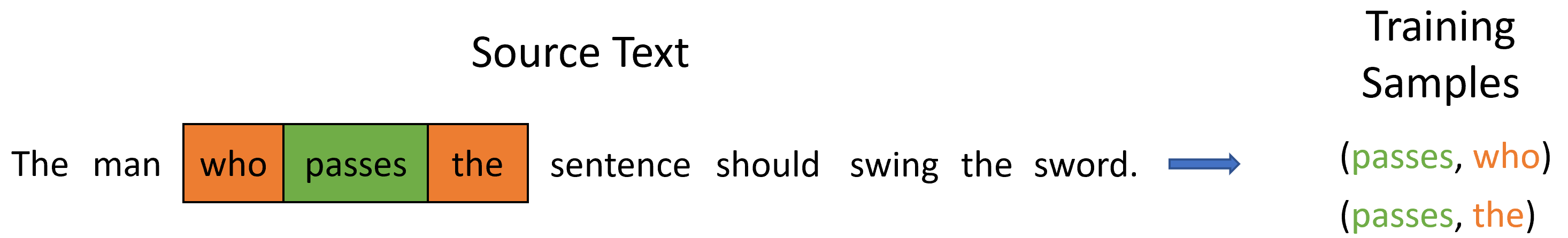
Figure 4: Training Window
For illustration purpose, a three-dimensional neural net will be constructed. In gensim, this can be implemented by setting size=3. This makes $N = 3$. Note that size is also a hyper-parameter that can be empirically tuned. In real life, a typical Word2Vec model has 200-600 neurons.
        from gensim.models import Word2Vec

        model = Word2Vec(corpus, size=3, window=1)
This means that the input weight matrix ($W_{input}$) will have a size of $8 \times 3$, and output weight matrix ($W_{output}^T$) will have a size of $3 \times 8$. Recall that the corpus, "The man who passes the sentence should swing the sword", has 8 unique vocabularies ($V = 8$).
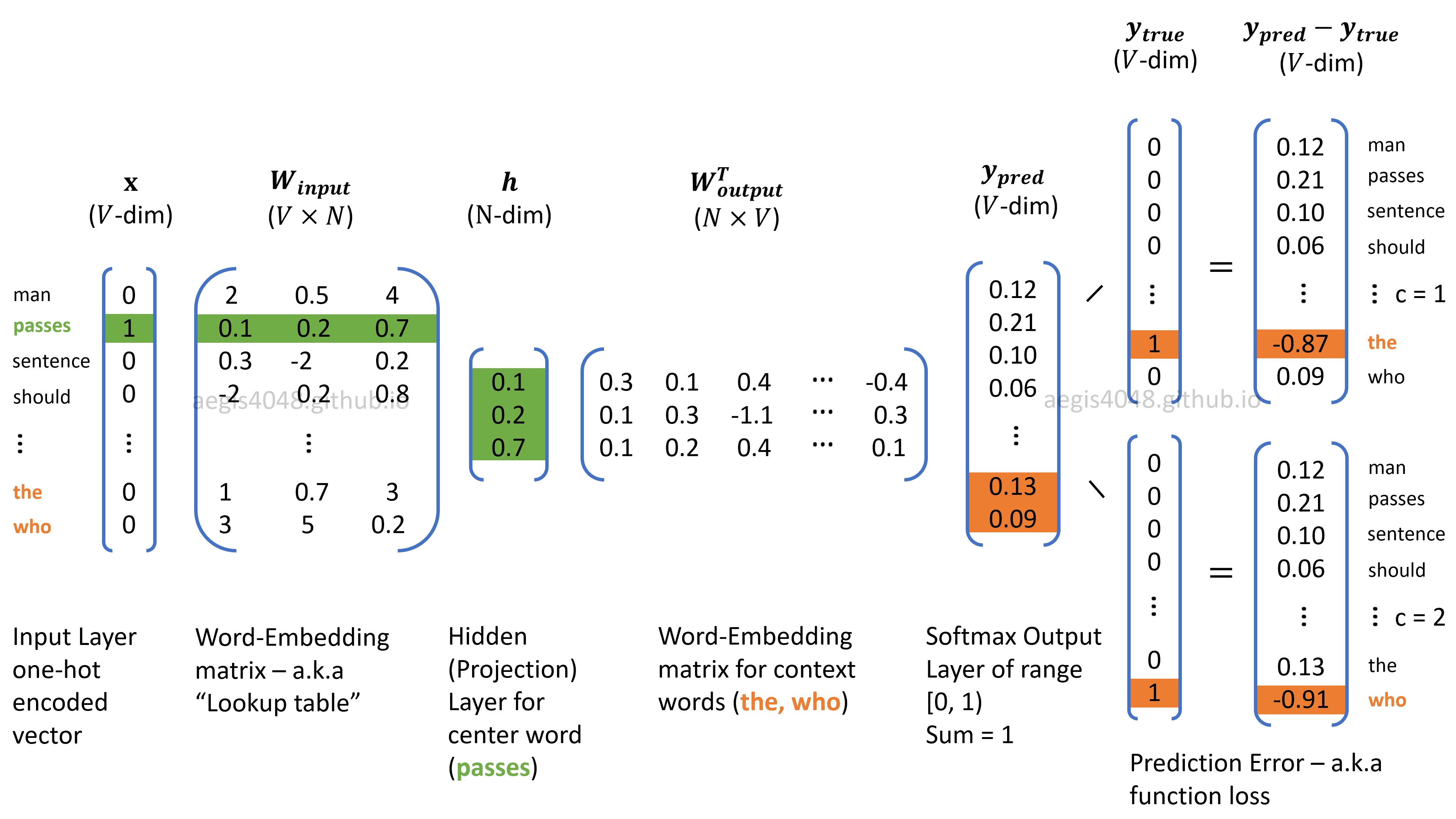
Figure 5: Skip-Gram model structure. Current center word is "passes"
5.1. Training: forward propagation
The word embedding matrices ($W_{input}$, $W_{output}$) in Skip-Gram are optimized through forward and backward propagations. For each iteration of forward + backward propagations, the model learns to reduce prediction error by optimizing the weight matrix ($\theta$), thus acquiring higher quality embedding matrices that better capture relationships among words.
Forward propagation includes obtaining the probability distribution of words ($y_{pred}$ in Figure 5) given a center word, and backward propagation includes calculating the prediction error, and updating the weight (embedding) matrices to minimize the prediction error.
5.1.1. Input layer ($x$)
The input layer is a $V$-dim one-hot encoded vector. Every element in the vector is 0 except one element that corresponds to the center (input) word. Input vector is multiplied with the input weight matrix ($W_{input}$) of size $V \times N$, and yields a hidden (projection) layer ($h$) of $N$-dim vector. Because the input layer is one-hot encoded, it makes the input weight matrix ($W_{input}$) to behave like a look-up table for the center word. Assuming epoch number of 1 (iter=1 in gensim Word2Vec implementation) and stochastic gradient descent, the input vector is injected into the network $T$ times for every word in the corpus and makes $T$ updates to the weight matrix ($\theta$) to learn from the training samples. Derivation of the stochasitc update equations are explained below.
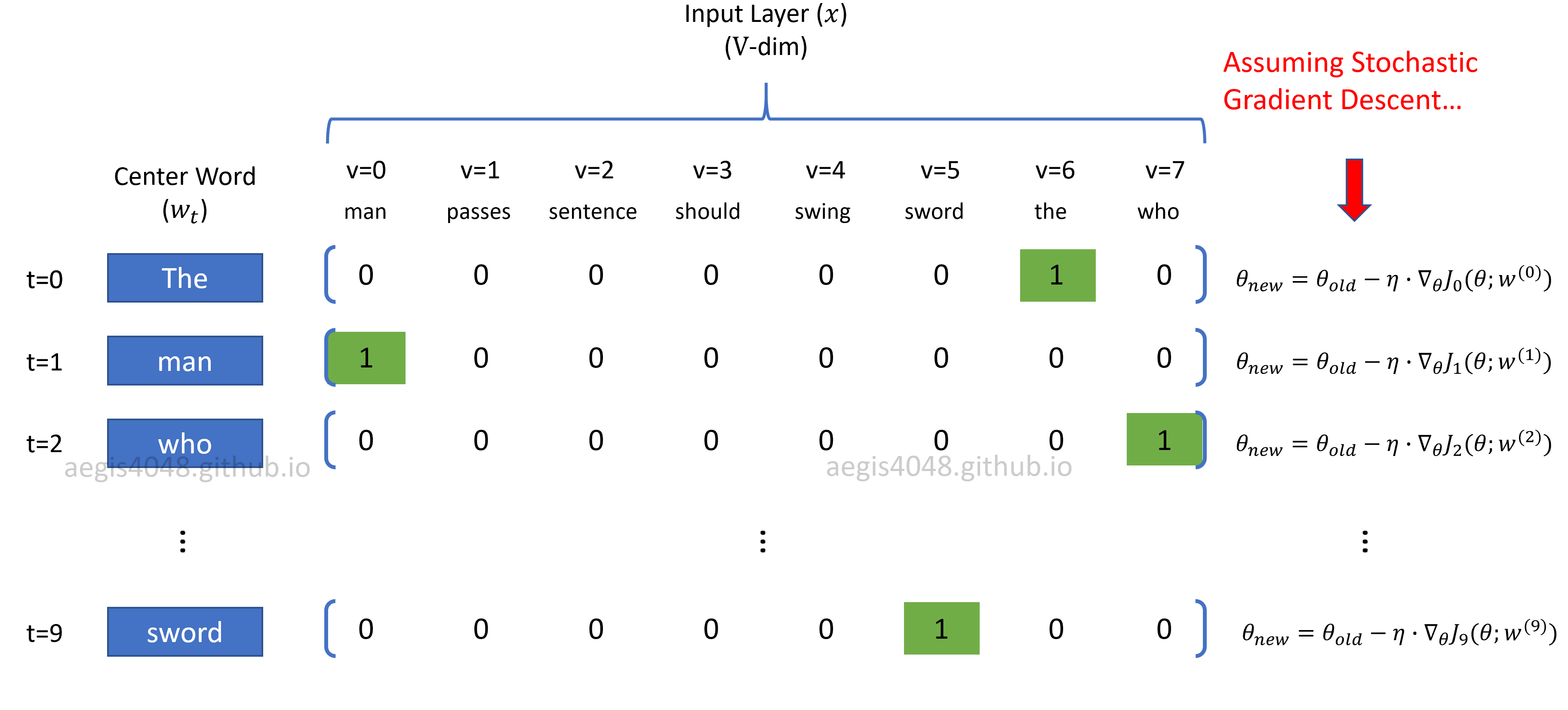
Figure 6: One-hot encoded input vector and parameter update
Notes: Stochastic gradient descent
The goal of any machine learning model is to find the optimal values of a weight matrix ($\theta$) to minimize prediction error. A general update equation for weight matrix looks like the following:
$\eta$ is learning rate, $\nabla_{J(\theta)}$ is gradient for the weight matrix, and $J(\theta)$ is the cost function that has different forms for each model. The cost function for the Skip-Gram model proposed in the Word2Vec original paper has the following equation:
Here, what gives us headache is the expression, $\frac{1}{T} \sum^T_{t=1}$, because $T$ can be larger than billions or more in many NLP applications. It is basically telling us that billions of iterations need to be computed to make just one update to the weight matrix ($\theta$). In order to mitigate this computational burden, the author of the paper states that Stochastic Gradient Descent (SGD) was used for parameter optimization. SGD removes the expression, $\frac{1}{T} \sum^T_{t=1}$, from the cost function and performs parameter update for each training example, $w^{(t)}$:
Then, the new parameter update equation for SGD becomes:
The original vanilla graident descent makes $1$ parameter update for $T$ training samples, but the new update equation using SGD makes $T$ parameter update for $T$ training samples. However, this comes at the price of higher fluctuation (or variance) in minimizing prediction error.
5.1.2. Input and output weight matrix ($W_{input}$, $W_{output}$)
Why does Skip-Gram model attempt to predict context words given a center word? How does predicting context words help with quantifying words and representing them in a vector space? In fact, the ultimate goal of the model is not to predict context words, but to construct the word embedding matrices ($W_{input}$, $W_{output}$) that best caputure relationship among words in a vector space. Skip-Gram achieves this by using a neural net — it optimizes the weight (embedding) matrices by adjusting the weight matrix to minimize the prediction error ($y_{pred} - y_{true}$). This will make more sense once you understand how the embedding matrix behaves like a look-up table.
Each row in a word-embedding matrix is a word-vector for each word. Consider the following word-embedding matrix, $W_{input}$.
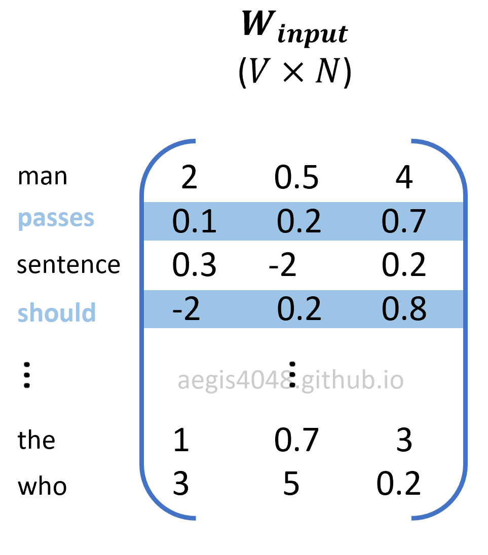
Figure 7: Word-embedding matrix, $W_{input}$
The words of our interest are "passes" and "should". "passes" has a word vector of $[0.1 \quad 0.2 \quad 0.7]$ and "should" has $[-2 \quad 0.2 \quad 0.8]$. Since we set the size of the weight matrix to be size=3, the matrix is three-dimensional, and can be visualized in a 3D vector space:
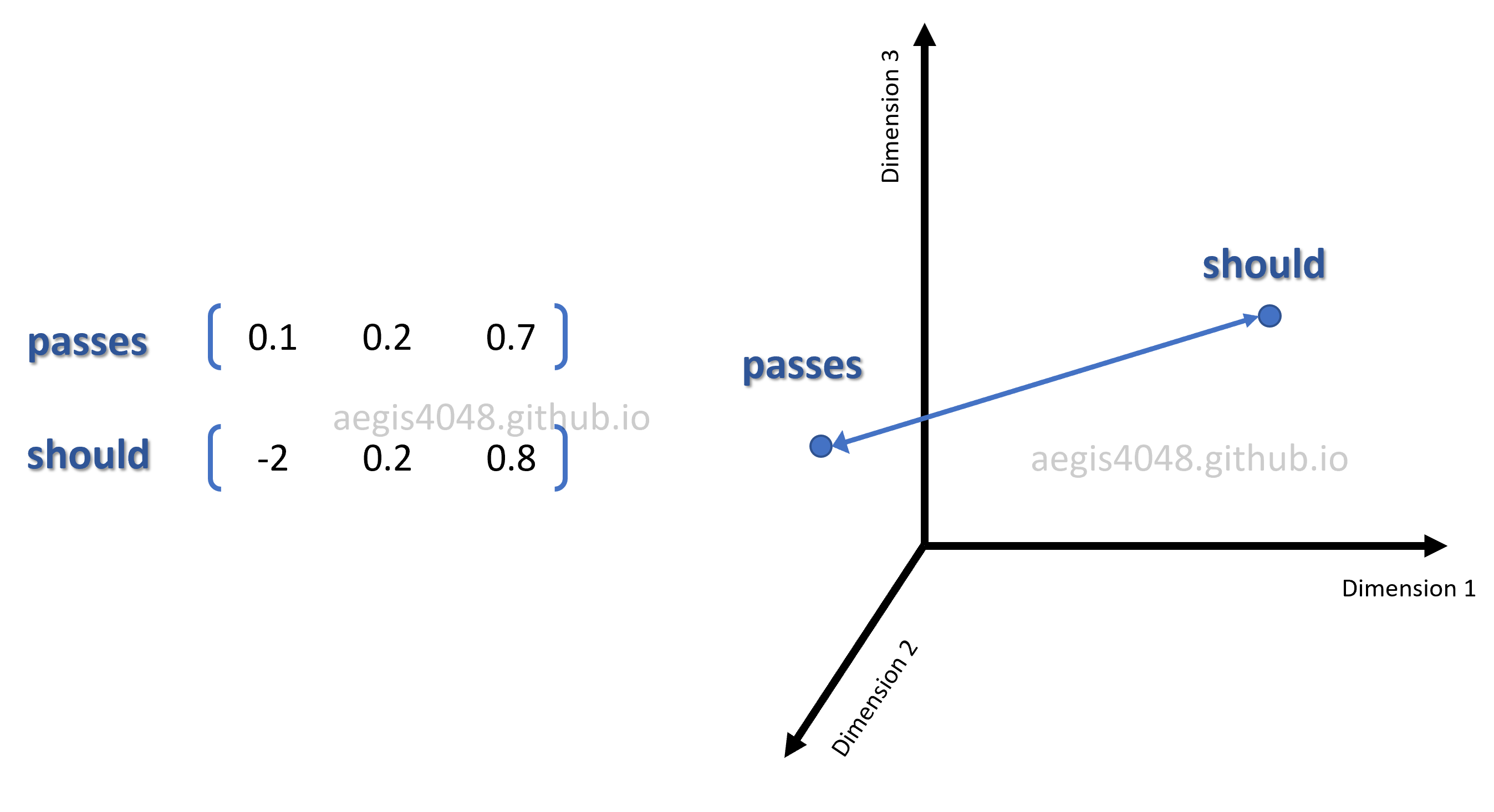
Figure 8: 3D visualization of word vectors in embedding matrix
Optimizing the embedding (weight) matrices $\theta$ results in representing words in a high quality vector space, and the model will be able to capture meaningful relationships among words.
Notes: $\theta$ in cost function
There are two weight matrices that need to be optimized in Skip-Gram model: $W_{input}$ and $W_{output}$. Often times in neural net, the weights are expressed as $\theta$. In Skip-Gram, $\theta$ is a concatenation of input and output weight matrices — $[W_{input} \quad W_{output}]$.
$\theta$ has a size of $2V \times N$, where $V$ is the number of unique vocab in a corpus, and $N$ is the dimension of word vectors in the embedding matrices. $2$ is multipled to $V$ because there are two weight matrices, $W_{input}$ and $W_{output}$. $u$ is a word vector from $W_{input}$ and $v$ is a word vector from $W_{output}$. Each word vectors are $N$-dim row vectors from input and output embedding matrices.
5.1.3. Hidden (projection) layer ($h$)
Skip-Gram uses a neural net with one hidden layer. In the context of natural language processing, hidden layer is often referred to as a projection layer, because $h$ is essentially an N-dim vector projected by the one-hot encoded input vector.
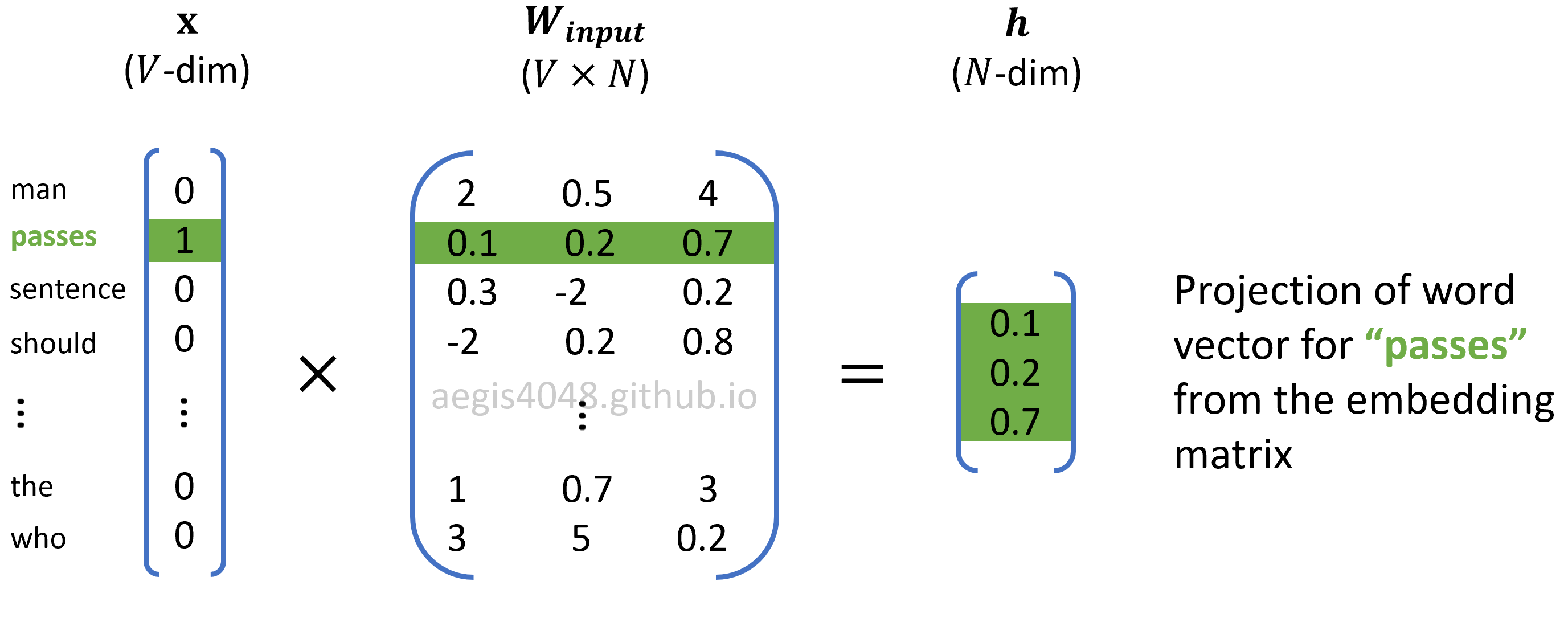
Figure 9: Computing projection layer
$h$ is obtained by multiplying the input word embedding matrix with the $V$-dim input vector.
5.1.4. Softmax output layer ($y_{pred}$)
The output layer is a $V$-dim probability distribution of all unique words in the corpus, given a center word. In statistics, the conditional probability of $A$ given $B$ is denoted as $p(A|B)$. In Skip-Gram, we use the notation, $p(w_{context}| w_{center})$, to denote the conditional probability of observing a context word given a center word. It is obtained by using the softmax function,
where $W_{output_{(i)}}$ is the $i$-th row vector of size $1 \times N$ from the output embedding matrix, $W_{output_{context}}$ is also a row vector of size $1 \times N$ from the output embedding matrix corresponding to the context word. $V$ is the size of unique vocab in the corpus, and $h$ is the hidden (projection) layer of size ($N \times 1$). The output is an $1 \times 1$ scalar value of probability of range $[0, 1)$.
This probability is computed $V$ times to obtain a conditional probability distribution of observing each unique vocabs in the corpus, given a center word.
$W_{output}$ in the denominator of eq 13 has size $V \times N$. Multiplying $W_{output}$ with $h$ of size $N \times 1$ will yield a dot product vector of size $V \times 1$. This dot product vector goes through the softmax function:
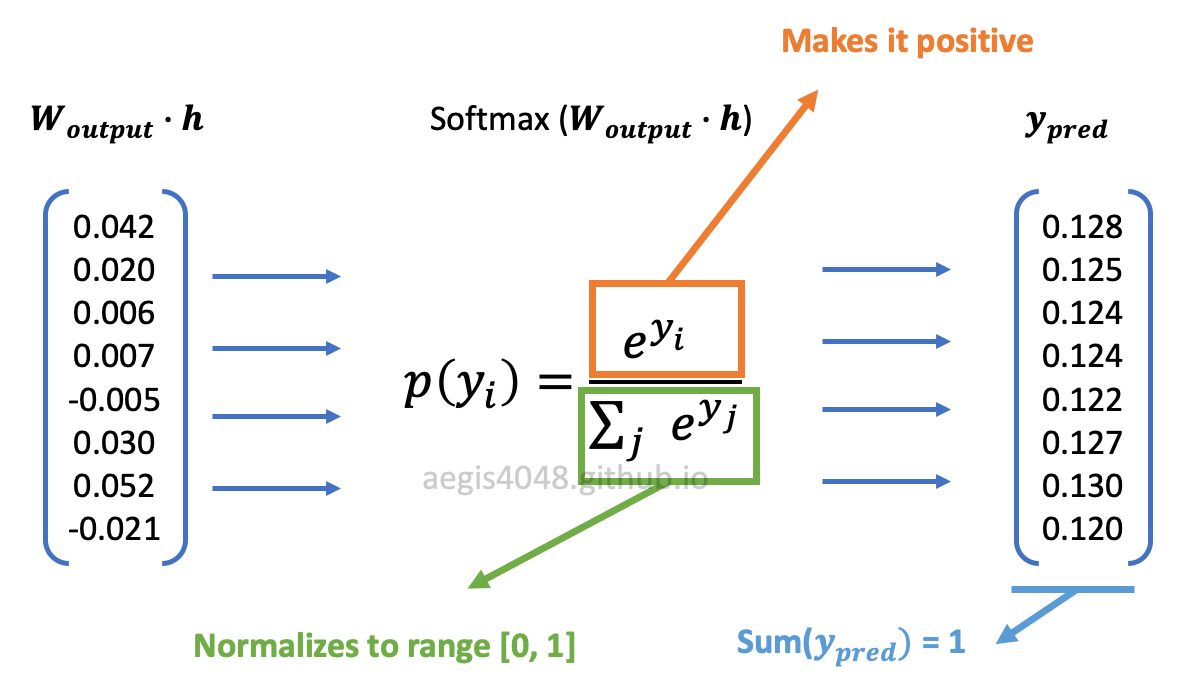
Figure 10: softmax function transformation
The exponentiation ensures that the transformed values are positive, and the normalization factor in the denominator ensures that the values have a range of $[0, 1)$. The result is a conditional probability distribution of observing each unique vocabs in the corpus, given a center word.
Notes: Negative sampling
Softmax function in Skip-Gram has the following equation:
There is an issue with softmax in Skip-Gram — it is computationally very expensive, as it requires scanning through the entire output embedding matrix ($W_{output}$) to compute the probability distribution of all $V$ words, where $V$ can be millions or more. Furtheremore, the normalization factor in the denominator also requires $V$ iterations. When implemented in codes, the normalization factor is computed only once and cached as a Python variable, making the alogrithm complexity = $O(V+V)\approx O(V)$.
Due to this computational inefficiency, softmax is not used in most implementaions of Skip-Gram. Instead we use an alternative called negative sampling with sigmoid function, which rephrases the problem into a set of independent binary classification task of algorithm complexity = $O(K+1)$, where $K$ typically has a range of $[5,20]$. Then, the new probability distribution is defined as:
$K=20$ is used for small corpus, and $K=5$ is used for big corpus. Negative sampling is much cheaper than vanilla Skip-Gram with softmax, because $K$ is between 5 ~ 20, whereas $V$ can be millions. Moreover, no extra iterations are necessary to compute the normalization factor in the denominator, because sigmoid function is a binary regression classifier. The algorithm complexity of the probability distribution of vanilla Skip-Gram is $O(V)$, whereas negative sampling's is $O(K+1)$. This shows why negative sampling saves a significant amount of computational cost per iteration.
In gensim, negative sampling is applied by default with Word2Vec(negative=5, ns_exponent=0.75), where negative is the number of $K$-negative samples, and ns_exponent is a hyperparameter related to negative sampling, of range $(0, 1)$. The details of the methodology behind negative sampling deserves another fully devoted post, and as such, covered in a different post.
5.2. Training: backward propagation
Backward propagation involves computing prediction errors, and updating the weight matrix ($\theta$) to optimize vector representation of words. Assuming stochastic gradient descent, we have the following general update equations for the weight matrix ($\theta$):
$\eta$ is learning rate, $\nabla_{J(\theta;w^{(t)})}$ is gradient for the weight matrix, and $J(\theta;w^{(t)})$ is the cost function defined in eq-6. Since the $\theta$ is a concatenation of input and output weight matrices ($[W_{input} \quad W_{output}]$) as described above, there are two update equations for each embedding matrix:
Mathematically, it can be shown that the gradients of $W_{input}$ $W_{output}$ have the following forms:
The gradients can be substitued into eq-16 and eq-17:
$W_{input}$ and $W_{output}$ are the input and output weight matrices, $x$ is one-hot encoded input layer, $C$ is window size, and $e_{c}$ is prediction error for $c$-th context word in the window. Note that $h$ (hidden layer) is equivalent to $W_{input}^T x$.
Notes: Applying Softmax
Although eq-21 does not explicitly show it, softmax function is applied in the prediction error ($e_c$). Prediction error is the difference between the predicted and true probability ($y_{pred} - y_{true}$) as illustrated below. The predicted probability $y_{pred}$ is computed using softmax function using eq-13.
5.1.1. Prediction error ($y_{pred} - y_{true}$)
Skip-Gram model optimizes the weight matrix ($\theta$) to reduce the prediction error. Prediction error is the difference between the probability distribution of words computed from the softmax output layer ($y_{pred}$) and the true probability distribution ($y_{true}$) of the $c$-th context word. Just like the input layer, $y_{true}$ is one-hot encoded vector, in which only one element in the vector that corresponds to the $c$-th context word is $1$, and the rest is all $0$.
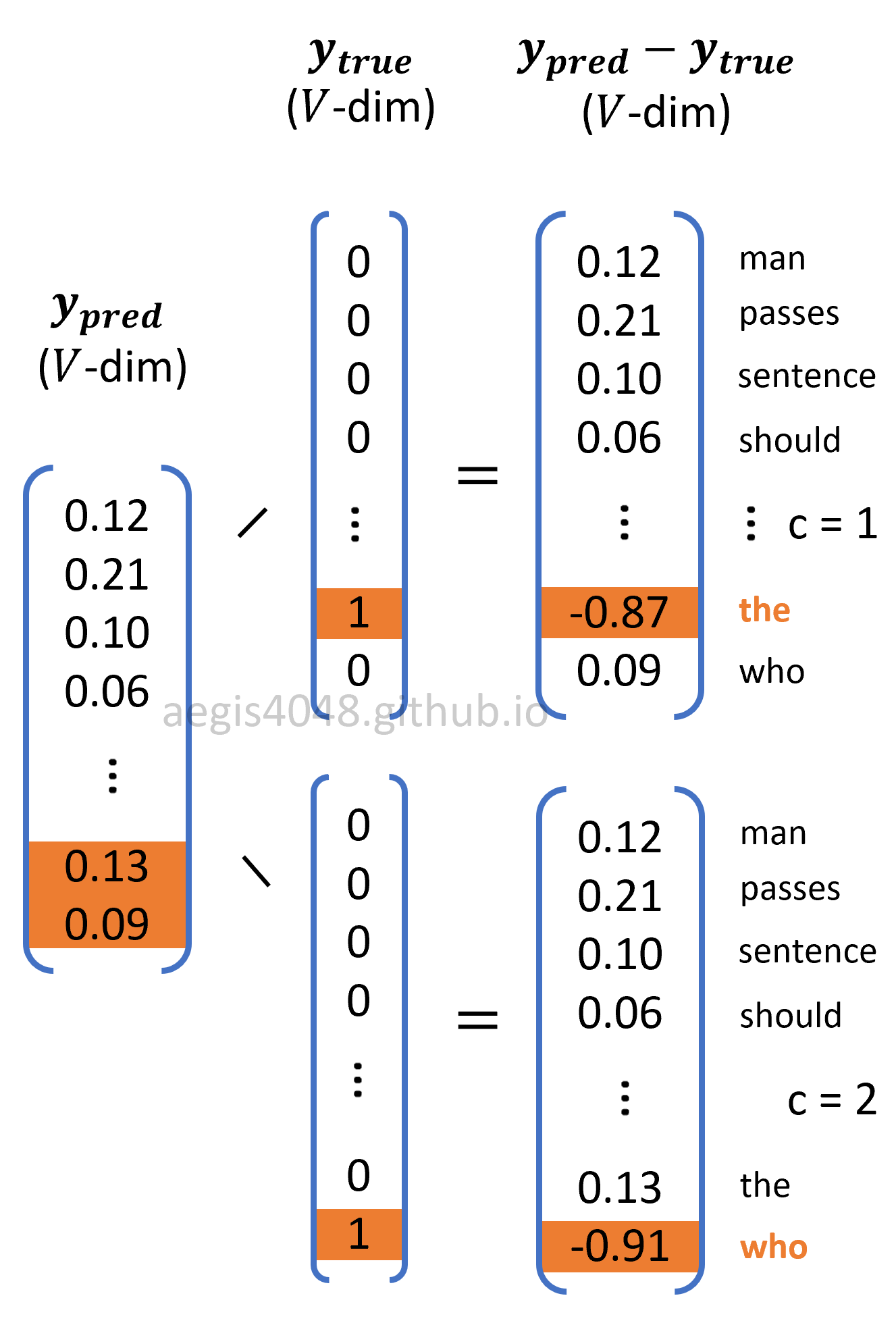
Figure 11: Prediction error window
The figure has a window size of $2$, so two prediction errors were computed. Recall from the above notes about the window size that the original softmax regression classifier (eq-10) has $K$ labels to classify, in which $K = V$ in NLP applications because there are $V$ words to classify. Employing window size transforms eq-10 into eq-11 significantly reduces the algorithm complexity because the model only needs to compute prediction errors for 2~10 (this is a hyperparameter $C$) neighboring words, instead of computing all $V$-prediction errors for all vocabs that can be millions or more.
Then, prediction errors for all $C$ context words are summed up to compute weight gradients to the update weight matrices, according to eq-18 and eq-19.
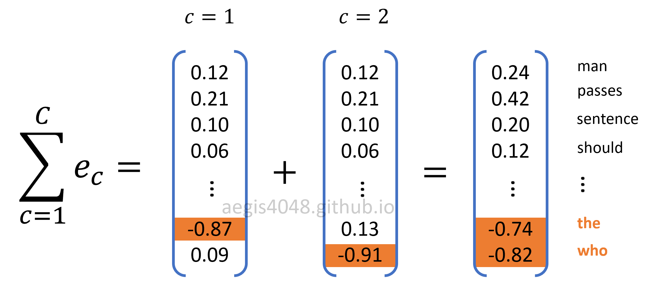
Figure 12: Sum of prediction errors
As the weight matrices are optimized, the prediction error for all words in the prediction error vector $\sum_{(c=1)}^C e_c$ converges to 0.
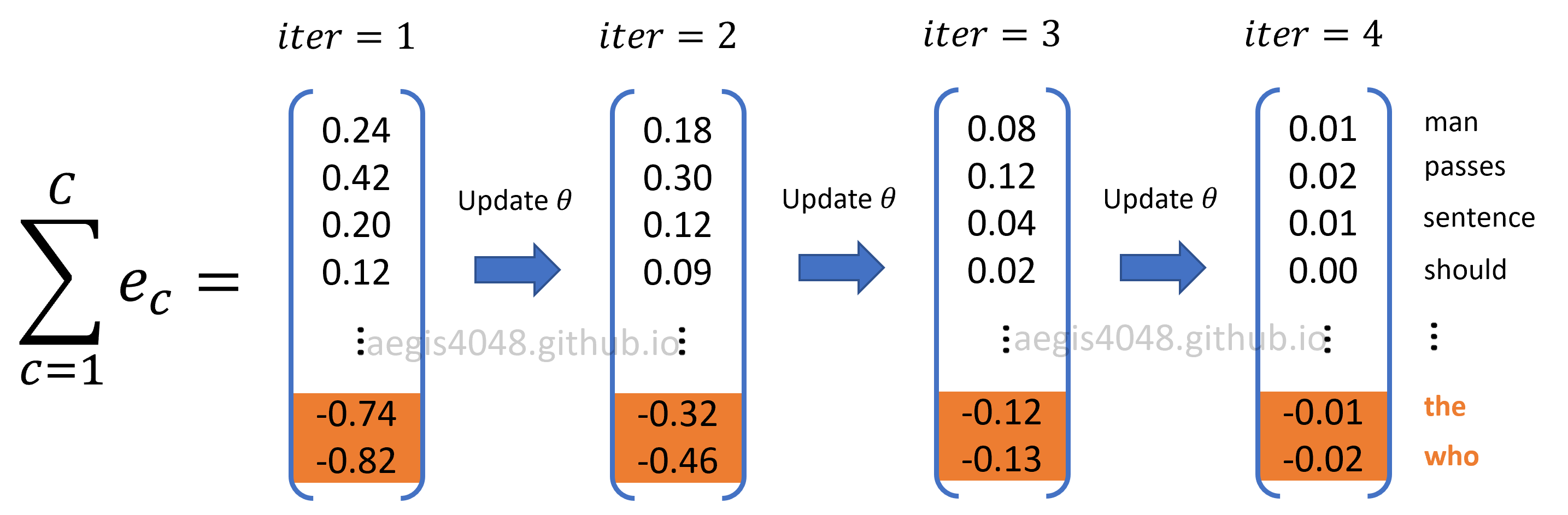
Figure 13: Prediction errors converging to zero with optimization
6. Numerical demonstration
For the ease of illustration, screenshots from Excel will be used to demonstrate the concept of updating weight matrices through forward and backward propagations.
Forward propagation: computing hidden (projection) layer
Center word is "passes". Window size is size=1, making "the" and "who" context words. Hidden layer ($h$) is looked up from the input weight matrix. It is computed with eq-12.
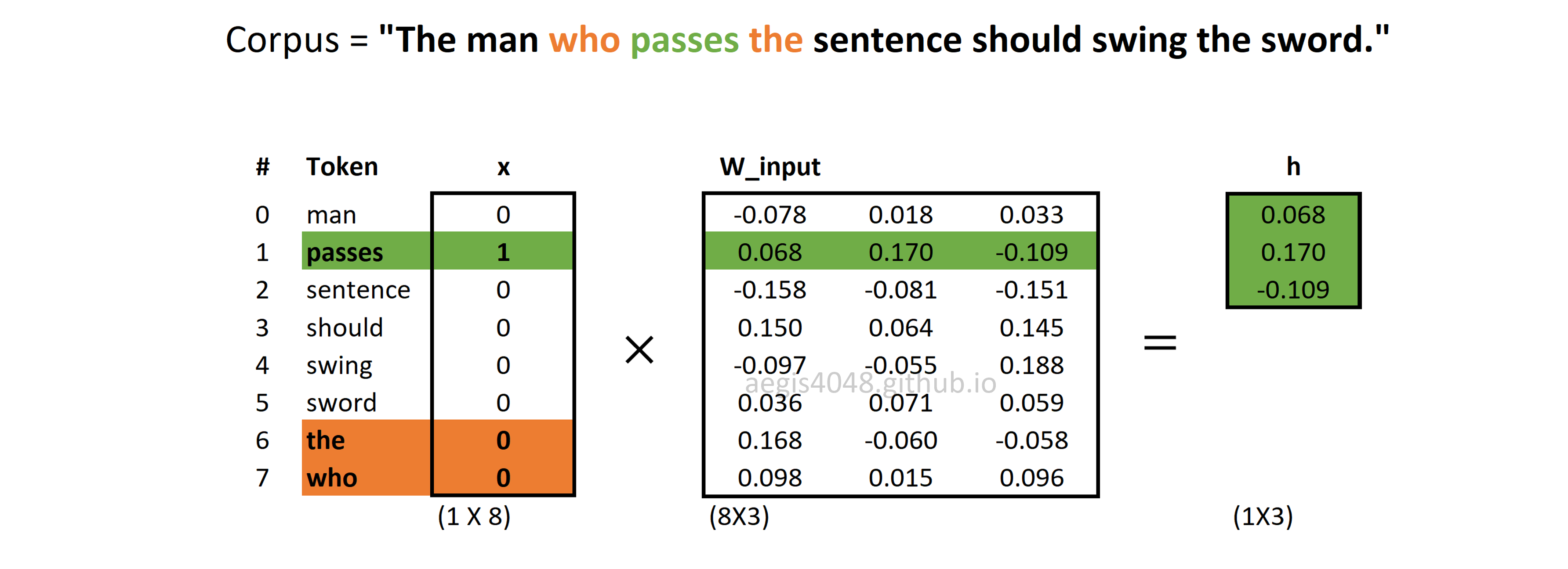
Figure 14: Computing hidden (projection) layer
Forward propagation: softmax output layer
Output layer is a probability distribution of all words, given a center word. It is computed with eq-14. Note that all context windows share the same output layer ($y_{pred}$). Only the errors ($e_c$) are different.
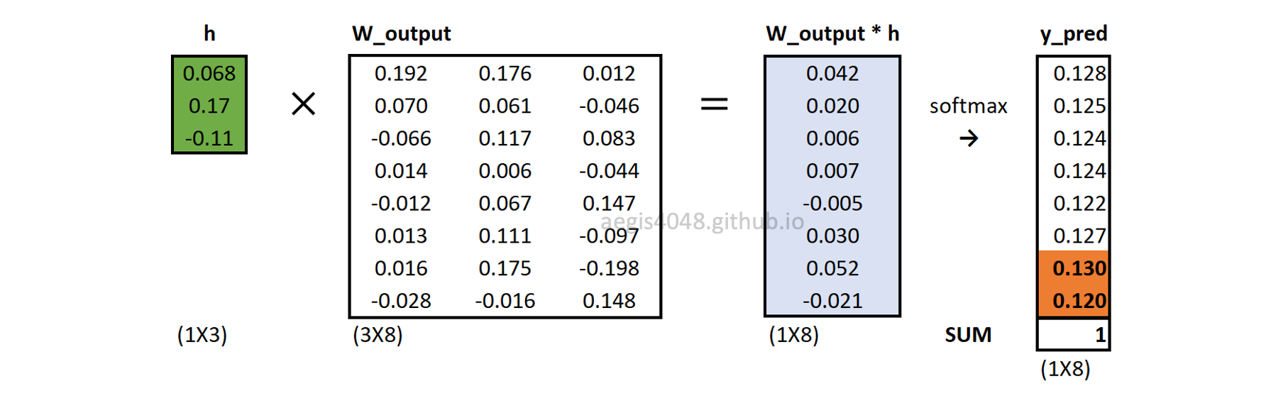
Figure 15: Softmax output layer
Backward propagation: sum of prediction errors
$C$ different prediction errors are computed, then summed up. In this case, since we set window=1 above, only two errors are computed.
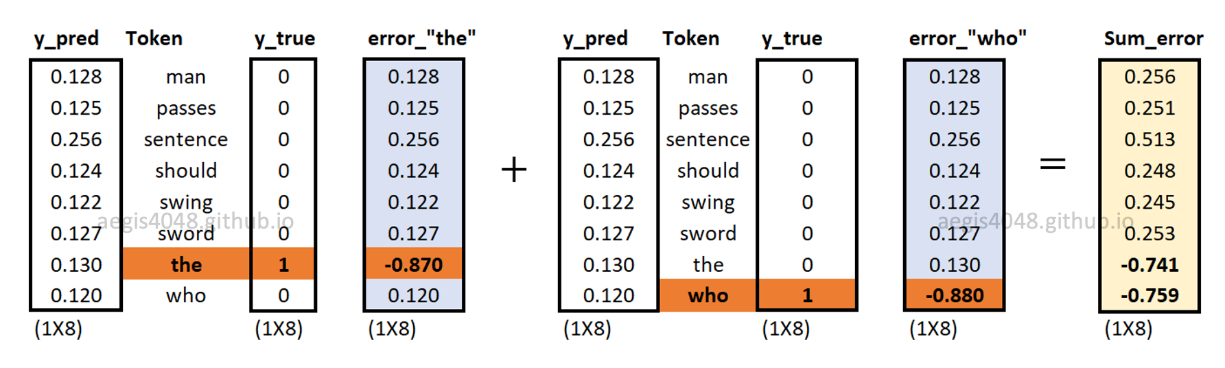
Figure 16: Prediction errors of context words
Backward propagation: computing $\nabla W_{input}$
Gradients of input weight matrix ($\frac{\partial J}{\partial W_{input}}$) are computed using eq-18. Note that multiplying $W_{output}^T \sum^C_{c=1} e_c$ with the one-hot-encoded input vector ($x$) makes the neural net to update only one word vector that corresponds to the input (center) word.
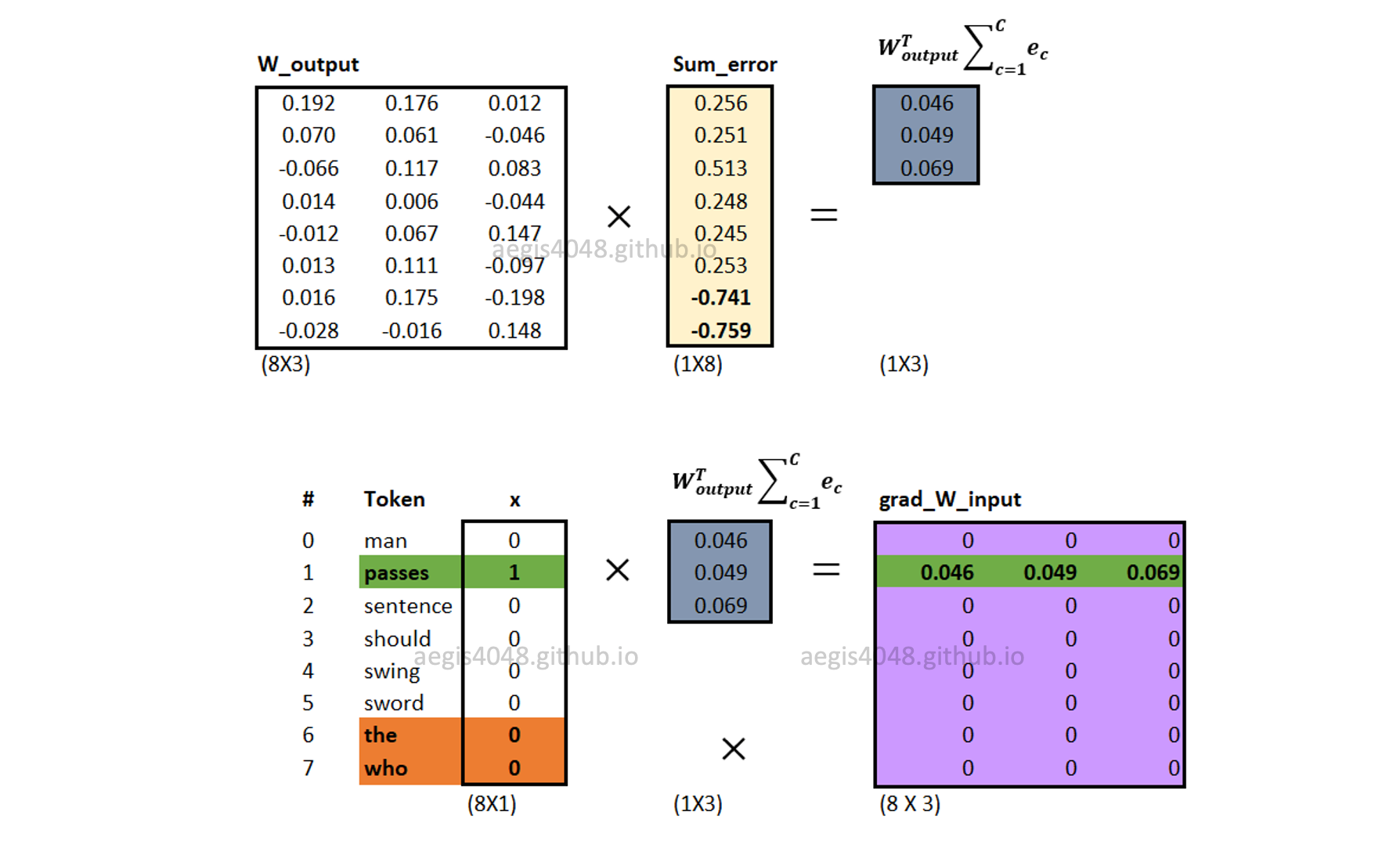
Figure 17: Computing input weight matrix gradient $\nabla W_{input}$
Backward propagation: computing $\nabla W_{output}$
Gradients of output weight matrix ($\frac{\partial J}{\partial W_{output}}$) are computed using eq-19. Unlike the input weight matrix ($W_{input}$), all word vectors in the output weight matrix ($W_{output}$) are updated.
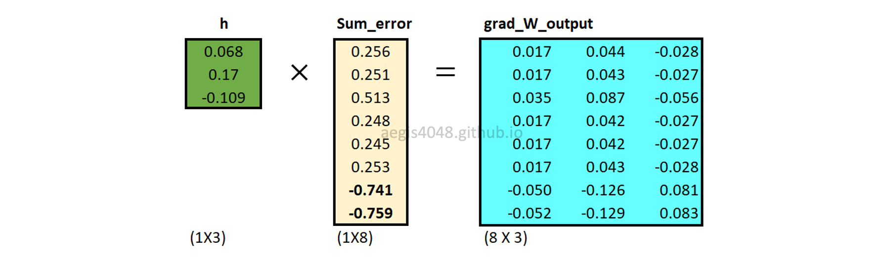
Figure 18: Computing output weight matrix gradient $\nabla W_{output}$
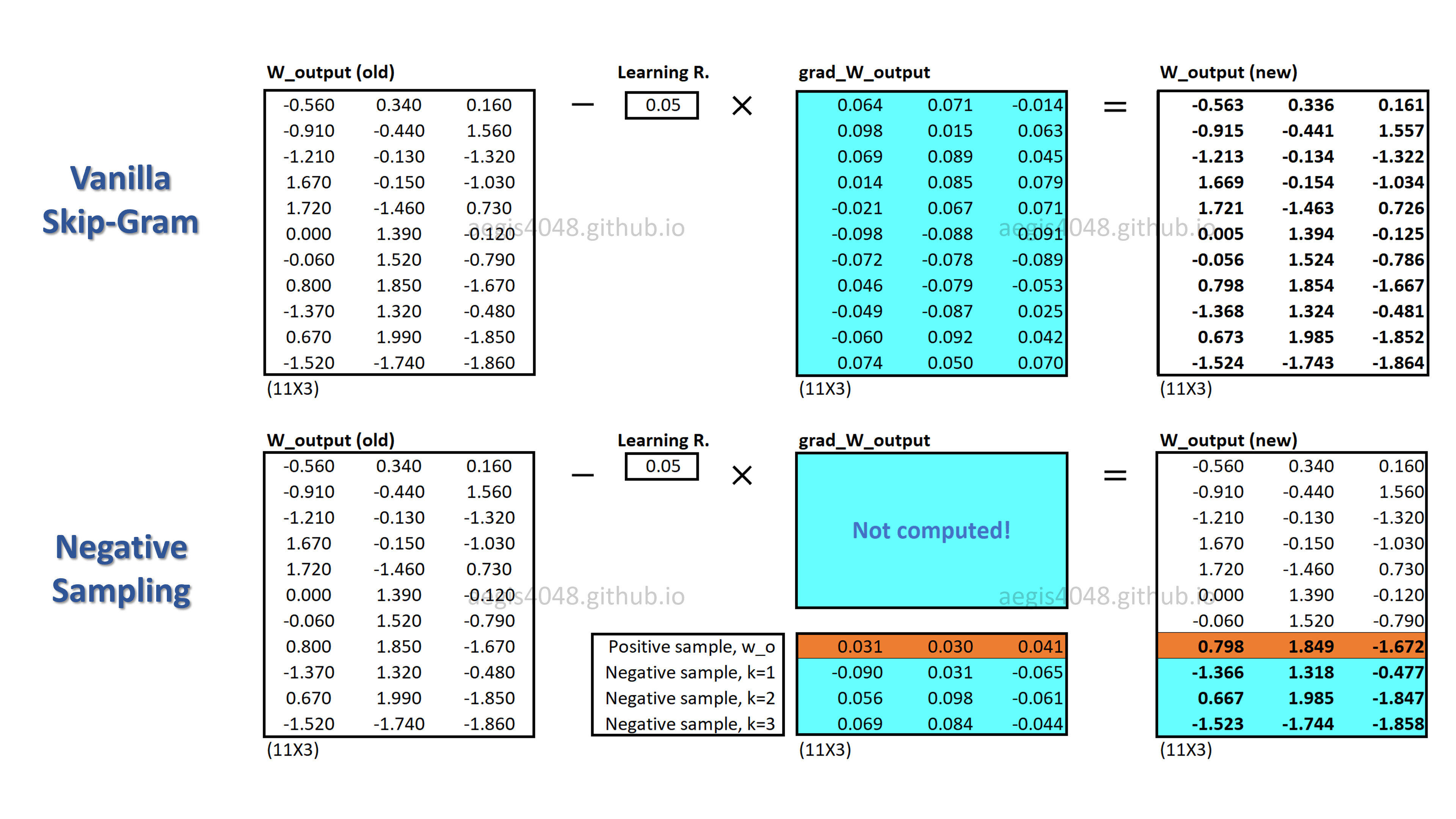
Backward propagation: updating weight matrices
Input and output weight matrices ($[W_{input} \quad W_{output}]$) are updated using eq-20 and eq-21.
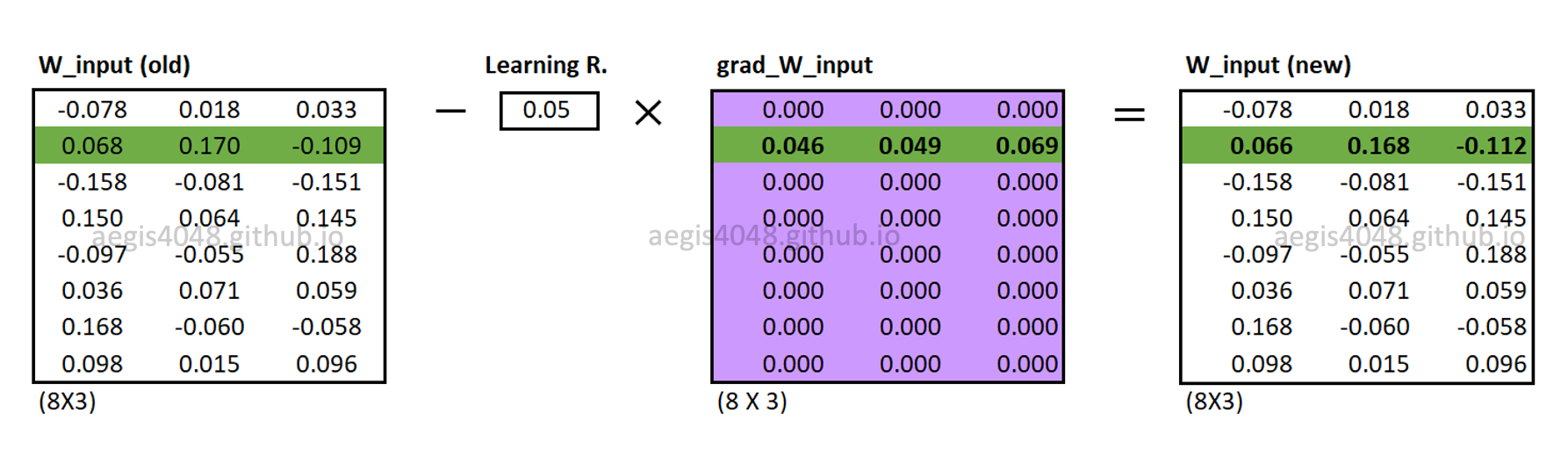
Figure 19: Updating $W_{input}$
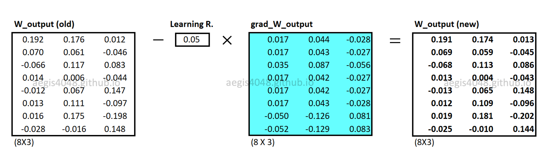
Figure 20: Updating $W_{output}$
Note that for each iteration in the learning process, all weights in $W_{output}$ are updated, but only one row vector that corresponds to the center word is updated in $W_{input}$. When the model finishes updating both of the weight matrices, then one iteration is completed. The model then moves to the next iteration with the next center word. However, remember that this uses eq-8 as the cost function and assumes stochastic gradient descent. This means that one update is made for each training example. If eq-9 is used as a cost function instead (which is almost never the case), then one update is made for all $T$ training examples in the corpus.
Related Posts
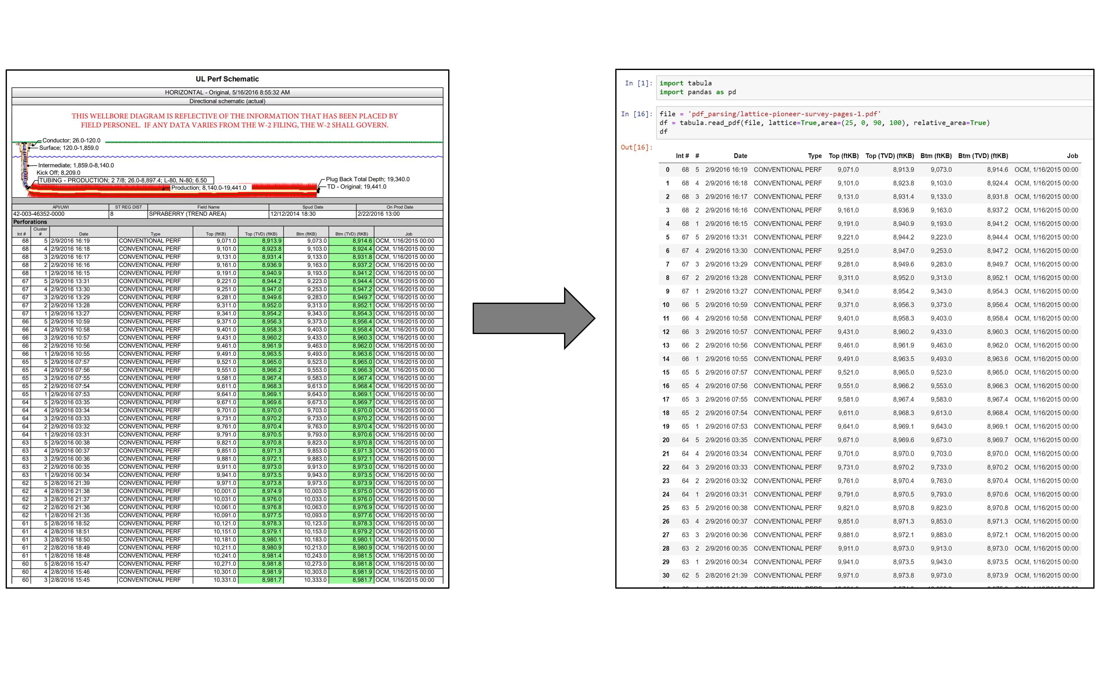
Parse PDF Files While Retaining Structure with Tabula-py
If you ever tried to do anything with data provided to you in PDFs, you know how painful it is — it's hard to copy-and-paste rows of data out of PDF files. Try tabula-py to extract data into a CSV or Excel spreadsheet using a simple, easy-to-use interface.
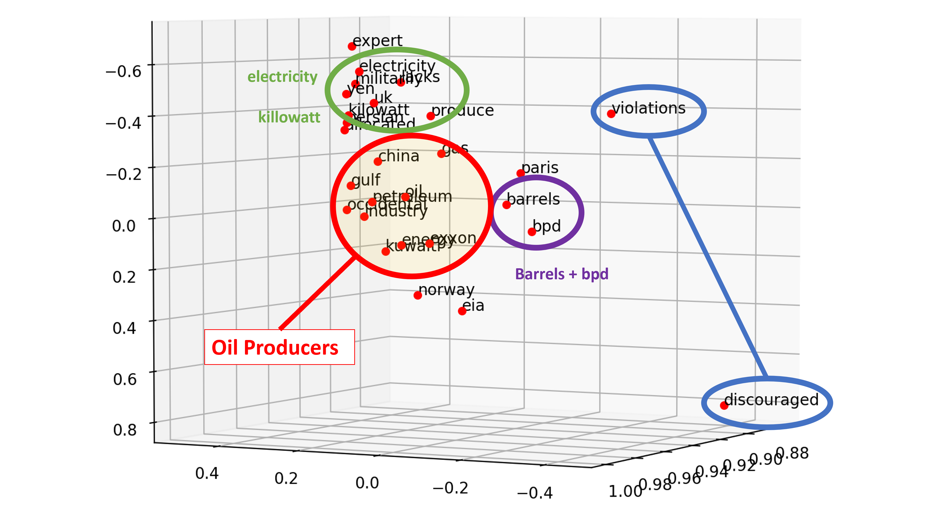
Understanding Multi-Dimensionality in Vector Space Modeling
How does word vectors in Natural Language Processing capture meaningful relationships among words? How can you quantify those relationships? Addressing these questions starts from understanding the multi-dimensional nature of NLP applications.
Optimize Computational Efficiency of Skip-Gram with Negative Sampling
When training your NLP model with Skip-Gram, the very large size of vocabs imposes high computational cost on your machine. Since the original Skip-Gram model is unable to handle this high cost, we use an alternative, called Negative Sampling.