GasCompressibility-py#
GasCompressibility-py is a Python library for calculating the gas compressibility factor, \(Z\), based on real gas law. It is designed with practical oil field application in mind, in which the required inputs (\(T\), \(P\), and \(\gamma_{g}\)) can be readily obtained from the surface facility.
The packages is under MIT License (no restrictions whatsoever).
1. Installation#
The package is hosted on the
PyPi page. You can
remotely install it with the pip command:
pip install gascompressibility
To download the most recent version:
pip install gascompressibility --upgrade
If you are a chemical or petroleum engineer who doesn’t know what
pip is, read below.
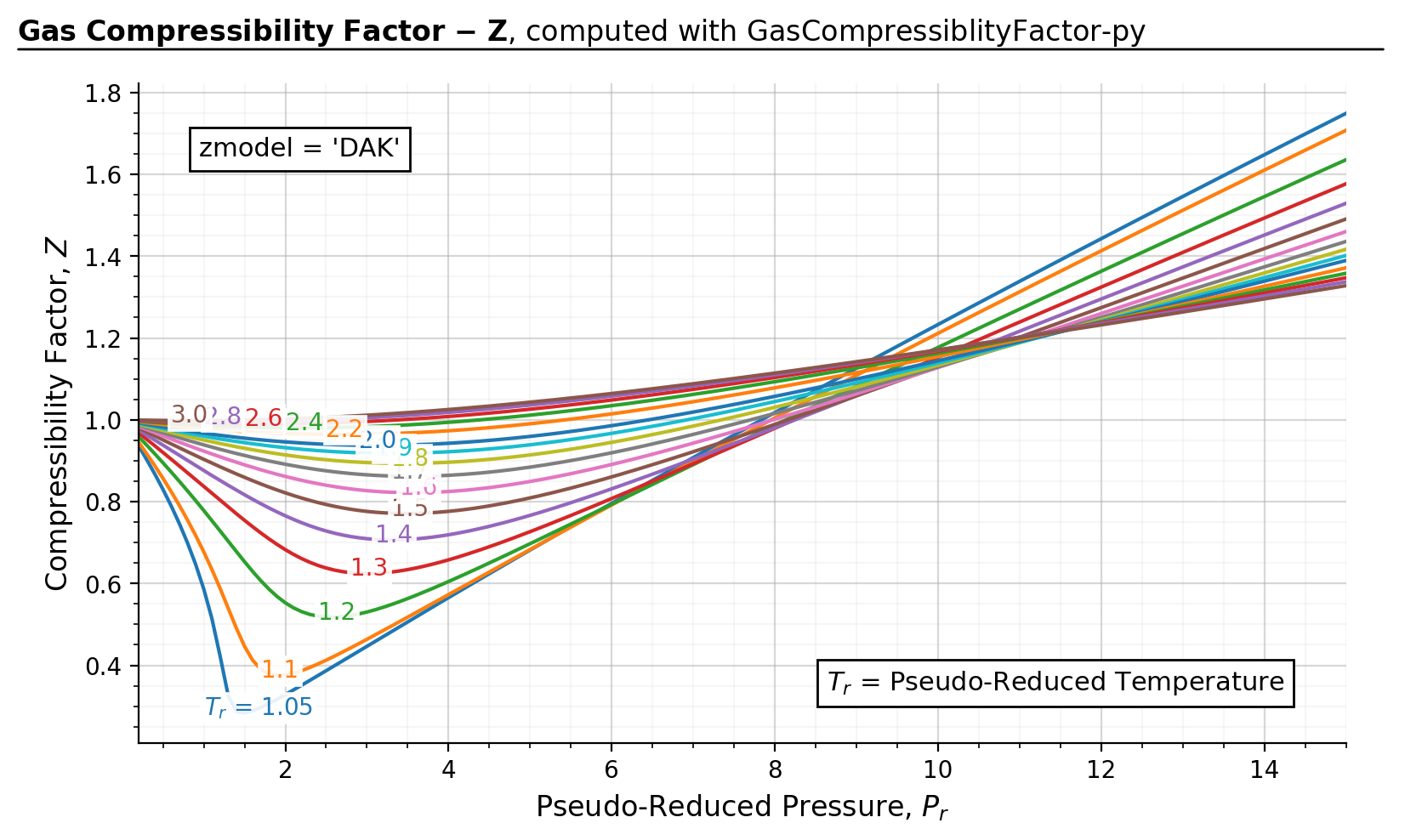
2. Quickstart#
Check gascompressibility.quickstart for more examples.
>>> import gascompressibility as gc
>>> import matplotlib.pyplot as plt
>>>
>>> results, fig, ax = gc.quickstart(prmin=0.2, prmax=15, zmodel='DAK')
>>> plt.show()

3. Usage#
The package allows for quick calculation of the z-factor from the gas specific gravity (\(\gamma_{g}\)), pressure (\(P\)), and temperature (\(T\)). Check gascompressibility.calc_z for more examples.
Basic (most common) usage:
>>> import gascompressibility as gc
>>>
>>> gc.calc_z(sg=0.7, T=75, P=2010)
0.7366562810878984
In presence of significant non-hydrocarbon impurities:
>>> gc.calc_z(sg=0.7, T=75, P=2010, CO2=0.1, H2S=0.07, N2=0.05)
0.7765149771306533
When pseudo-critical properties are known (not common):
>>> gc.calc_z(Pr=1.5, Tr=1.5)
0.859314380561347
Picking correlation models of your choice
>>> gc.calc_z(sg=0.7, T=75, P=2010, zmodel='kareem', pmodel='sutton')
0.7150183342641309
Returning all associated pseudo-critical properties computed
>>> gc.calc_z(sg=0.7, T=75, P=2010, ps_props=True)
{'z': 0.7366562810878984, 'Tpc': 371.4335560823552, 'Ppc': 660.6569792741872, 'J': 0.56221847, 'K': 14.450840999999999, 'Tr': 1.4394768357478496, 'Pr': 3.0646766226921294}
The package additionally supports calculation of pseudo-critical properties. Check gascompressibility.pseudocritical.Sutton and gascompressibility.pseudocritical.Piper for more information.
Reduced pressure calculation from specific gravity:
>>> from gascompressibility.pseudocritical import Piper
>>>
>>> Piper().calc_Pr(sg=0.7)
2.7950877932259734
Pseudo-critical pressure calculation from specific gravity:
>>> Piper().calc_Ppc(sg=0.7, N2=0.1, CO2=0.1, H2S=0.05)
724.3779622618493
Reduced pressure calculation from pseudo-critical pressure
>>> Sutton().calc_Pr(Ppc=724.37, P=2010)
2.7951185167800987
4. Models Implemented#
Pseudo-critical models:
Sutton (1985): Makes corrections for acid fractions: \(H_2S\) and \(CO_2\)
Piper (1993): Improved version of Piper. Additionally supports corrections for \(N_2\) along with \(H_2S\) and \(CO_2\)
Z-factor models:
DAK (1975): The most widely used z-factor model in the oil and gas industry for the past 40 years. You can’t go wrong with this model
Hall-Yarborough (1973): Not recommended.
Londono (2005): Improved version of DAK. Math is exactly the same, but regression coefficients are fitted with 4x more data points.
Kareem (2016): Fast, but have shorter working ranges (\(P_r < 15\))
Not sure which model to use? You don’t need to worry about it - default models (Piper + DAK) are more than good enough for real life applications. However, if computation speed is a big concern, use Kareem’s method for z-factor correlation for \(P_r < 15\). Check Theories 3: What models should I use? for more information.
5. Working Ranges#
The below table summarizes the working \(P_r\) and \(T_r\) ranges of each model, according to it’s own original paper.
Model |
\(P_r\) |
\(T_r\) |
|---|---|---|
DAK |
[1, 3] |
[0.2, 30] |
Hall-Yarborough |
[1.15, 3] |
(0, 20.5] |
Londono |
[1, 3] |
[0.2, 30] |
Kareem |
[1.15, 3] |
[0.2, 15] |
something
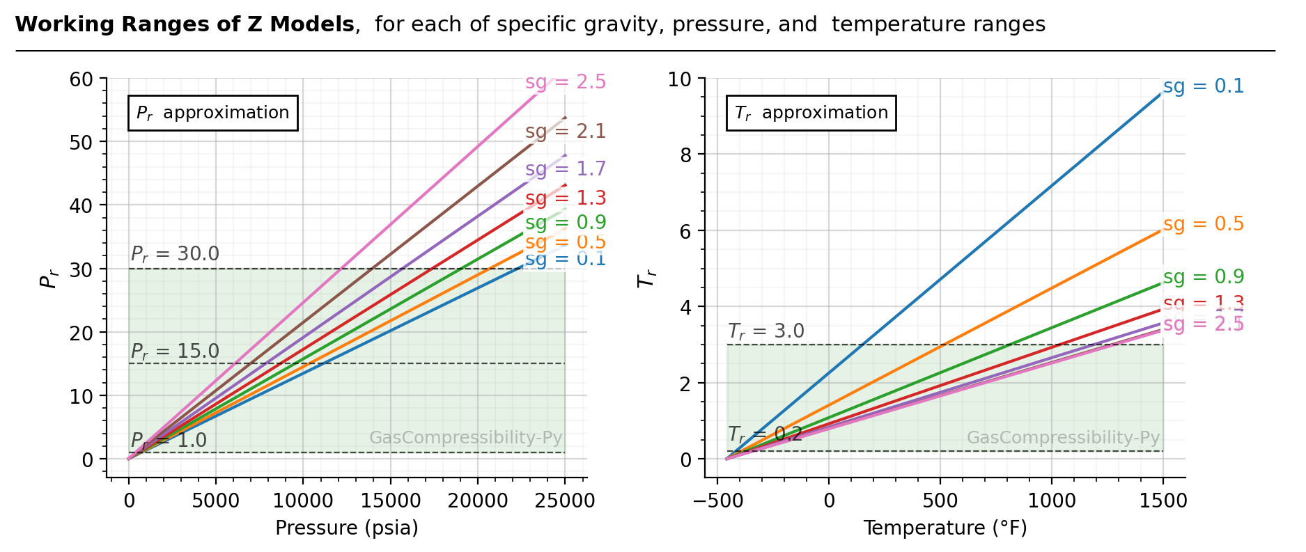
However, normally we don’t know the \(P_r\) and \(T_r\) values of a given mixture. The below figure summarizes
the corresponding \(P_r\) and \(T_r\) (computed with Sutton’s method) for each of specific gravity, temperature, and pressure ranges. For
example, assuming \(\gamma_{g}\) = 0.9 (green lines), z-factor correlation can’t be used for extreme conditions like
\(P\) > 19,000 psia, or \(T\) > 800 °F. If Kareem’s method (zmodel='kareem') is used for speed, you can’t
use it for \(P\) > 11,500 psia.

Figure source code
import matplotlib.pyplot as plt
import numpy as np
from gascompressibility.pseudocritical import Sutton

pmin = 0
pmax = 25000
Ps = np.linspace(pmin, pmax, 100)
Ps = np.array([round(P, 1) for P in Ps])

tmin = -459
tmax = 1500
Ts = np.linspace(tmin, tmax, 100)
Ts = np.array([round(T, 1) for T in Ts])

sgs = np.arange(0.1, 2.6, 0.4)
sgs = np.array([round(sg, 1) for sg in sgs])

results = {sg: {
    'Pr': np.array([]),
    'P': np.array([]),
    'Tr': np.array([]),
    'T': np.array([]),
} for sg in sgs}

for sg in sgs:
    for P in Ps:
        Pr = Sutton().calc_Pr(sg=sg, P=P)
        results[sg]['P'] = np.append(results[sg]['P'], [P], axis=0)
        results[sg]['Pr'] = np.append(results[sg]['Pr'], [Pr], axis=0)
    for T in Ts:
        Tr = Sutton().calc_Tr(sg=sg, T=T)
        results[sg]['T'] = np.append(results[sg]['T'], [T], axis=0)
        results[sg]['Tr'] = np.append(results[sg]['Tr'], [Tr], axis=0)

fig, axes = plt.subplots(1, 2, figsize=(9, 4))
for i, ax in enumerate(axes):
    if i == 0:
        for sg in sgs:
            Prs = results[sg]['Pr']
            Ps = results[sg]['P']

            p = ax.plot(Ps, Prs, label=sg)

            t = ax.text(Ps[-10], max(Prs) - 3, 'sg = ' + str(sg), color=p[0].get_color())
            t.set_bbox(dict(facecolor='white', alpha=0.7, edgecolor='white', pad=1))

        ax.text(0.06, 0.9, '$P_{r}$  approximation', fontsize=9, transform=ax.transAxes,
            bbox=dict(facecolor='white'))
        ax.set_ylabel('$P_r$', fontsize=11)
        ax.set_xlabel('Pressure (psia)')
        ymax = 60
        ax.hlines(y=30, xmin=pmin, xmax=pmax, color='k', linestyle='--', linewidth=0.8, alpha=0.7)
        ax.text(100, 31.3, '$P_r$ = 30.0', alpha=0.7)
        ax.hlines(y=15, xmin=pmin, xmax=pmax, color='k', linestyle='--', linewidth=0.8, alpha=0.7)
        ax.text(100, 16, '$P_r$ = 15.0', alpha=0.7)
        ax.hlines(y=1, xmin=pmin, xmax=pmax, color='k', linestyle='--', linewidth=0.8, alpha=0.7)
        ax.text(100, 2, '$P_r$ = 1.0', alpha=0.7)
        ax.fill_between(x=Ps, y1=1, y2=30, color='green', interpolate=True, alpha=0.1, zorder=-99)

    else:
        for sg in sgs:
            Trs = results[sg]['Tr']
            Ts = results[sg]['T']

            p = ax.plot(Ts, Trs, label=sg)

            t = ax.text(Ts[-1], max(Trs), 'sg = ' + str(sg), color=p[0].get_color())
            t.set_bbox(dict(facecolor='white', alpha=0.7, edgecolor='white', pad=1))

        ax.text(0.06, 0.9, '$T_{r}$  approximation', fontsize=9, transform=ax.transAxes,
            bbox=dict(facecolor='white'))
        ax.set_ylabel('$T_r$', fontsize=11)
        ax.set_xlabel('Temperature (°F)')
        ymax = 10
        ax.hlines(y=3, xmin=tmin, xmax=tmax, color='k', linestyle='--', linewidth=0.8, alpha=0.7)
        ax.text(tmin, 3.2, '$T_r$ = 3.0', alpha=0.7)
        ax.hlines(y=0.2, xmin=tmin, xmax=tmax, color='k', linestyle='--', linewidth=0.8, alpha=0.7)
        ax.text(tmin, 0.5, '$T_r$ = 0.2', alpha=0.7)
        ax.fill_between(x=Ts, y1=0.2, y2=3, color='green', interpolate=True, alpha=0.1, zorder=-99)


    ymin = 0 - 0.05 * ymax
    ax.set_ylim(ymin, ymax)

    ax.minorticks_on()
    ax.grid(alpha=0.5)
    ax.grid(visible=True, which='minor', alpha=0.1)
    ax.spines.top.set_visible(False)
    ax.spines.right.set_visible(False)


    def setbold(txt):
        return ' '.join([r"$\bf{" + item + "}$" for item in txt.split(' ')])

    bold_txt = setbold('Working Ranges of Z Models')
    plain_txt = ',  for each of specific gravity, pressure, and  temperature ranges'

    fig.suptitle(bold_txt + plain_txt,
                 verticalalignment='top', x=0, horizontalalignment='left', fontsize=11)
    yloc = 0.9
    ax.annotate('', xy=(0.01, yloc), xycoords='figure fraction', xytext=(1.02, yloc),
                arrowprops=dict(arrowstyle="-", color='k', lw=0.7))
    ax.text(0.95, 0.1, 'GasCompressibility-Py', fontsize=9, ha='right', va='center',
            transform=ax.transAxes, color='grey', alpha=0.5)

fig.tight_layout()
6. Tips#
What does ‘pip’ mean?
If you are asking this question, you are probably a petroleum or chemical engineer with minimal programming knowledge. It’s basically a command-line program that helps you download & install any open-source library with minimal hassle. Here I offer some practical tips for engineers not proficient in Python (yet…!):
Download Anaconda from here.
Run the downloaded file. It’s filename will look something like this: “Anaconda3-2023.03-1-Windows-x86_64.exe”
It will ask you to select destination folder. By default, its
C:\ProgramData\Anaconda3If it asks you to check if you want to add Codna to the environtment PATH variable, check yes. It will say that it is not recommended, but trust me - this will make your life easier if you don’t know what you are doing.
Once installation is finished, go to windows search tab (bottom left corner of your screen). Type “cmd” and launch.
If installation is done correctly, you should have
(base)next to your current directory, like this:(base) C:\Users\EricKim>. If you don’t see(base), go to windows search tab again. Type “Anaconda”. Click “Anaconda Prompt (Anaconda 3)” and launch it. If you still don’t see(base), you are about to do dive into some painful troubleshooting. Ask your friends who are good at Python to help you with it.If the Anaconda installation is done correctly, make your command line look like the following and press enter:
(base) C:\Users\EricKim>pip install gascompressibility.Congrats! Installation is finished
Type
(base) C:\Users\EricKim>Jupyter Notebookand try the package on Jupyter Notebook.
7. References#
[1] Sutton, R.P.: “Compressibility Factor for High-Molecular Weight Reservoir Gases,” paper SPE 14265 (1985). (link)
[2] Piper, L.D., McCain Jr., W.D., and Corredor J.H.: “Compressibility Factors for Naturally Occurring Petroleum Gases,” paper SPE 26668 (1993). (link)
[3] Dranchuk, P.M., and Abou-Kassem, J.H.: “Calculation of z-Factors for Natural Gases Using Equations of State,” Journal of Canadian Petroleum Technology (1975). (link)
[4] Kay, W.B: “Density of Hydrocarbon Gases and Vapors at High Temperature and Pressure,” Industrial Engineering Chemistry (1936)
[5] Wichert, E.: “Compressibility Factor of Sour Natural Gases,” MEng Thesis, The University of Calgary, Alberta (1970)
[6] Stewart, W.F., Burkhardt, S.F., and Voo, D.: “Prediction of Pseudocritical Parameters for Mixtures,” paper presented at the AIChE Meeting, Kansas City, MO (May 18, 1959).
[7] Hall, K.R., and Yarborough, L.: “A new equation of state for Z-factor calculations,” Oil and Gas Journal (1973). (link)
[8] Londono, F.E., Archer, R.A., and Blasingame, T.A.: “Simplified Correlations for Hydrocarbon Gas Viscosity and Gas Density — Validation and Correlation of Behavior Using a Large-Scale Database,” paper SPE 75721 (2005). (link)
[9] Kareem, L.A., Iwalewa, T.M., and Marhoun, M.al-.: “New explicit correlation for the compressibility factor of natural gas: linearized z-factor isotherms,” Journal of Petroleum Exploration and Production Technology (2016). (link)
[10] Elsharkawy, A.M., Aladwani, F., Alostad, N.: “Uncertainty in sour gas viscosity estimation and its impact on inflow performance and production forecasting,” Journal of Natural Gas Science and Engineering (2015). (link)
[11] Elsharkawy, A.M.: “Predicting the Properties of Sour Gases and Condensates: Equations of State and Empirical Correlations,” paper SPE 74369 (2002). (link)
[12] Elsharkawy, A.M., and Elsharkawy, L.: “Predicting the compressibility factor of natural gases containing various amounts of CO2 at high temperatures and pressures,” Journal of Petroleum and Gas Engineering (2020). (link)
8. Requirements#
Python => 3.9
Numpy
Scipy
Matplotlib
10. Cite As#
Eric “Soobin” Kim, 2021, GasCompressibility-py Python Package, PyPI, Python Package Index, https://pypi.org/project/gascompressibility/.