Theories#
The goal of all existing z-factor correlation models is to numerically represent the famous Standing-Katz (SK) chart, correlating the pseudo-critical properties, reduced pressure (\(P_{r}\)) and reduced temperature (\(T_{r}\)), to the real gas compressibility factor \(Z\). In the other words, calculation of the z-factor requires values of \(P_{r}\) and \(T_{r}\).
In real life applications, no one knows the exact \(P_{r}\) and \(T_{r}\) values of his gas mixture. This is where pseudo-critical property models, such as Sutton (1985) [1] and Piper et al (1993) [2], comes in handy by approximating them from gas specific gravity (\(\gamma_g\)), which is relatively easy to obtain from lab sample analysis.
This section explains the basic theories behind \(P_{r}\) and \(T_{r}\) correlation from specific gravity and the subsequent z-factor correlation from the computed \(P_{r}\) and \(T_{r}\).
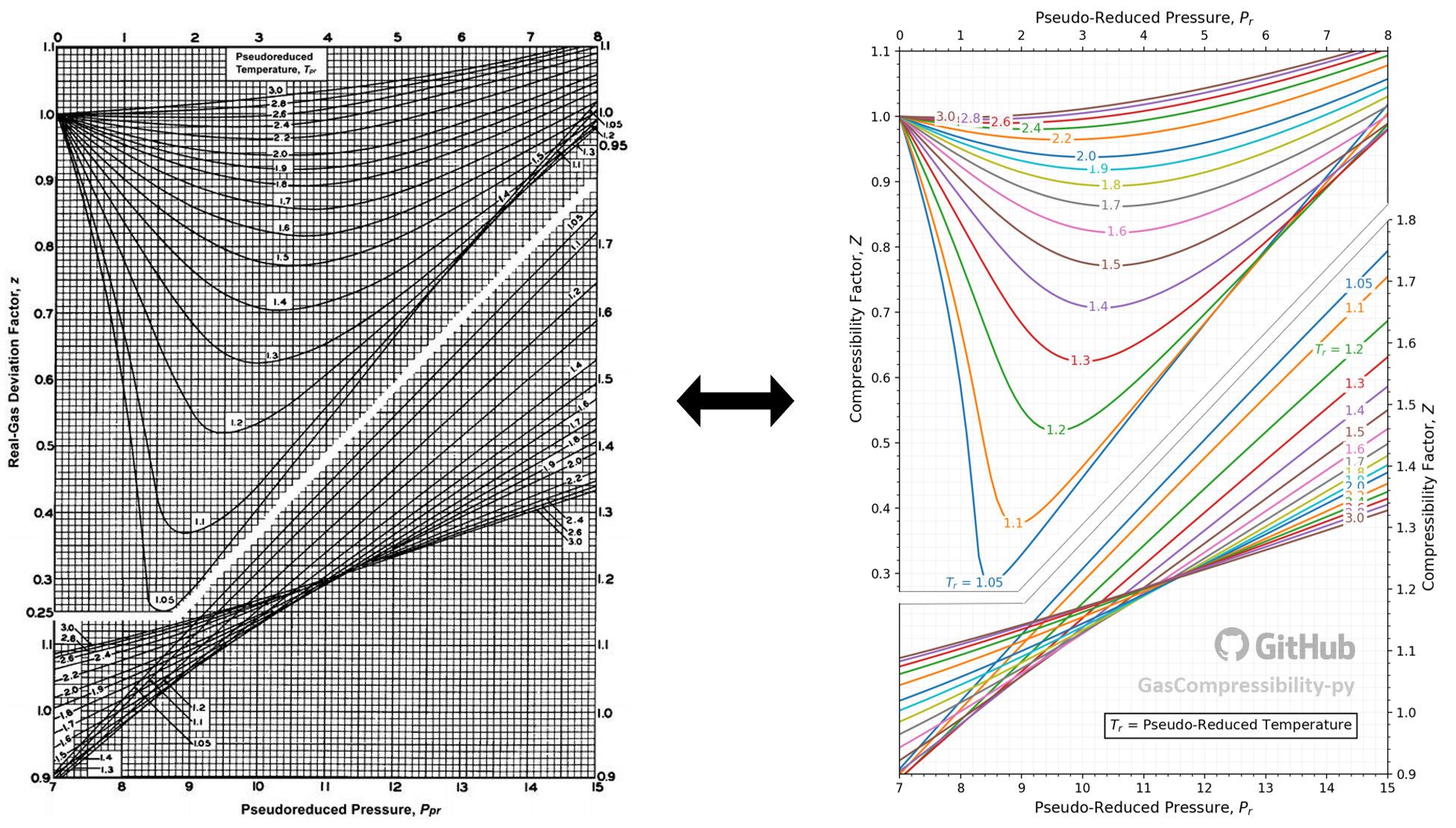
Figure 1: Left is the original SK chart, and the right is the numerical representation of the SK chart using the Dranchuk and Abu-Kassem (DAK) model [3].
1. Pseudo-Critical Property Models#
The z-factor can be derived from \(P_{r}\) and \(T_{r}\) through visual inspection of the SK chart or through numerical computation using various z-factor correlation models. In the other words, z-factor is a function of pseudo-reduced pressure and temperature:
\(P_{r}\) and \(T_{r}\) are defined as the pressure and temperature divided by the mixture’s pseudo-critical pressure (\(P_{pc}\)) and and temperature (\(T_{pc}\)):
Kay (1936) [4] stated that \(P_{pc}\) and \(T_{pc}\) of a gas mixture can be expressed as the mole fraction (\(x\)) weighted average of the critical pressure (\(P_c\)) and temperature (\(T_c\)) of the mixture’s individual component (\(i\)):
However, this method is too inconvenient because you have to manually input individual component’s \(P_c\), \(T_c\), and \(x\), which can be time-consuming. Furthermore, this isn’t practical for oil field applications in which the lab analysis of the “heavy-ends” are often lumped up together and reported as \(C_{6}^{+}\) or \(C_{7}^{+}\). This makes it impossible to know the mole fractions of the components heavier than \(C_{6}\) or \(C_{7}\).
This section introduces various pseudo-critical property models that correlates a gas mixture’s specific gravity (\(\gamma_{g}\)) to its corresponding \(P_{pc}\) and \(T_{pc}\).
1.1. Sutton (1985)#
Sutton (1985) [1] fitted the following regression model for a gas mixture with unknown component composition that that take \(\gamma_{g}\) as input:
The above correlations are valid over the ranges of specific gravities with which Sutton worked: \(0.57 < \gamma_{g} < 1.68\). He also recommends to apply Wichert-Aziz [5] correction for significant \(H_2S\) and \(CO_2\) fractions:
where:
\(\epsilon\) = temperature-correction factor for acid gases [°R]
\(A\) = sum of the mole fractions of \(CO_2\) and \(H_2S\) in the gas mixture [dimensionless]
\(B\) = mole fraction of \(H_2S\) in the gas mixture [dimensionless]
\(T^{'}_{pc}\) = corrected pseudo-critical temperature [°R]
\(P^{'}_{pc}\) = corrected pseudo-critical pressure [psia]
The correction correlation is applicable to concentration ranges of \(CO_2 < 54.4 \space mol\)% and \(H_2S < 73.8 \space mol\)%. Using the Dranchuk and Abu-Kassem (DAK) method [3] as a z-factor correlation model, Sutton’s correlation model reported an average absolute error of 1.418%. The regression coefficients were fitted with 289 points.
1.2. Piper et al. (1993)#
Piper et al. (1993) [2] adapted the method of Stewart et al. (1959) [6] to calculate the pseudo-critical properties of gas mixtures with nitrogen (\(N_2\)), \(CO_2\), and \(H_2S\) fractions:
and
where:
\(J\) = Steward, Burkhardt, and Voo (SBV) parameter [°R/psia]
\(K\) = SBV parameter [°R/psia^0.5]
\(x_{H_2S}\) = mole fraction of \(H_2S\) [dimensionless]
\(x_{CO_2}\) = mole fraction of \(CO_2\) [dimensionless]
\(x_{N2}\) = mole fraction of \(N_2\) [dimensionless]
Piper’s correction for non-hydrocarbon impurities have working ranges of \(H_2S < 51.37 \space mol\)%, \(CO_2 < 67.16 \space mol\)%, and \(N_2 < 15.68 \space mol\)%. Using the DAK method [3] as a z-factor correlation model, Piper’s crrelation model reported an average absolute error of 1.304%. The regression coefficients were fitted with 896 points.
1.3. Caveats#
1) The models work only for “naturally occurring” hydrocarbon gases
The models implemented in this library correlates \(\gamma_{g}\) to the corresponding \(P_{pc}\) and \(T_{pc}\) by using the fitted regression coefficients. This means that the working range of the models will be limited by the range of the data points used to fit the coefficients. All pseudo-critical models (that I know of) are developed using only the naturally occurring gas samples. Therefore, it is not recommended to use these models for synthetic gases. If you are dealing with synthetic gases, I recommend using Kay’s (1936) [4] method.
2) Correction is necessary in presence of significant impurities fractions
Sutton’s method (1985) [1] can apply correction for \(H_{2}S\) and \(CO_2\):
>>> from gascompressibility.pseudocritical import Sutton
>>>
>>> Sutton().calc_Tr(sg=0.7, T=75, CO2=0.1, H2S=0.07)
1.5005661019949397
Piper’s method (1993) [2] can apply correction for \(H_{2}S\), \(CO_2\), and \(N_2\):
>>> from gascompressibility.pseudocritical import Piper
>>>
>>> Piper().calc_Tr(sg=0.7, T=75, CO2=0.1, H2S=0.07, N2=0.1)
1.5483056093175225
2. Z-Factor Correlation Models#
There are two kinds of models for z-factor correlation: Implicit vs. Explicit models
Implicit models require iterative convergence to find the root of
non-linear equations. From the Python point of view, this means that
they use scipy.optimize.newton() method. These models are
computationally much more expensive than explicit models. However,
providing a good initial guess for the z-factor can significantly reduce
computational cost. Initial guess of \(Z = 0.9\) is a good starting
point for most applications in the oil field. This can be done by
setting calc_z(guess=0.9) in this library (however, this is unnecessary if you set
smart_guess=True).
Models implemented:
Explicit models require only 1 iteration. They are fast. These models tend to be restricted by smaller applicable \(P_{r}\) and \(T_{r}\) ranges and be less accurate than implicit models. It is important to check the working ranges of the parameters before implementing these models.
Models implemented:
Kareem, Iwalewa, and Marhoun (2016) [9]
2.1. DAK (1975)#
This method requires iterative converge. The z-factor is computed by setting \(z\) as the root of the following non-linear equations:
and
where:
\(A_{1} = 0.3265 ~~~~~~~~~ A_{2} = -1.0700 ~~~~~~~~~ A_{3} = -0.5339\)
\(A_{4}= 0.01569 ~~~~~~~ A_{5} = -0.05165 ~~~~~~~ A_{6} = 0.5475\)
\(A_{7} = -0.7361 ~~~~~~ A_{8} = 0.1844 ~~~~~~~~~~~~ A_{9} = 0.1056\)
\(A_{10} = 0.6134 ~~~~~~~~ A_{11} = 0.7210\)
The model’s tested working ranges are: \(1 \leq T_{r} \leq 3\) and \(0.2 \leq P_{r} \leq 30\). The regression coefficients were fitted on 1500 points. An average absolute error of 0.468% is reported in the original paper.
This method is widely used in the petroleum industry [10].
Code usage example:
>>> import gascompressibility as gc
>>> gc.calc_z(Pr=3.1995, Tr=1.5006)  # default: model='DAK'
0.7730934971021096
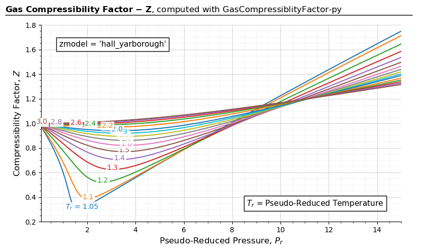
2.2. Hall-Yarborough (1973)#
This method requires iterative converge. The z-factor is computed by setting \(z\) as the root of the following non-linear equations:
and
where:
\(A_{1} = 0.06125te^{-1.2(1-t)^{2}}\)
\(A_{2}=14.76t - 9.76t^{2} + 4.58t^{3}\)
\(A_{3} = 90.7t - 242.2t^{2} + 42.4t^{3}\)
\(A_{4} = 2.18 + 2.82t,\)
\(t = 1 / T_{r}\),
The model’s tested working ranges are: \(1.15 < T_{r} \leq 3\) and \(0 < P_{r} \leq 20.5\). The regression coefficients were fitted with 289 points. An average absolute error of 1.21% is reported in the original paper.
This method has received great application in the natural gas industry [11].
Code usage example:
>>> import gascompressibility as gc
>>> gc.calc_z(zmodel='hall_yarborough', Pr=3.1995, Tr=1.5006)
0.77140002684377
2.3. Londono (2005)#
Londono’s method is exactly the same as the DAK method, and requires iterative converge. The only difference is that Londono further optimized the eleven regression coefficients by using more data points. DAK used 1500 points. Londono used 5960 points. The new regression coefficients are as follows:
\(A_{1} = 0.3024696 ~~~~~~~~~~ A_{2} = -1.046964 ~~~~~~~~~~ A_{3} = -0.1078916\)
\(A_{4}= -0.7694186 ~~~~~~~ A_{5} = 0.1965439 ~~~~~~~~~~~ A_{6} =0.6527819\)
\(A_{7} = -1.118884 ~~~~~~~~~ A_{8} = 0.3951957 ~~~~~~~~~~~ A_{9} = 0.09313593\)
\(A_{10} = 0.8483081 ~~~~~~~~~ A_{11} = 0.7880011\)
The original paper does not mention any tested working ranges of \(P_{r}\) and \(T_{r}\). However, it is logical to assume it’s working ranges to be the same as the those of the DAK method, \(1 \leq T_{r} \leq 3\) and \(0.2 \leq P_{r} \leq 30\), since the underlying math is the same. An average absolute error of 0.412% is reported in the original paper.
Code usage example:
>>> import gascompressibility as gc
>>> gc.calc_z(zmodel='londono', Pr=3.19, Tr=1.5)
0.7752626795793716
2.4. Kareem, Iwalewa, and Marhoun (2016)#
This method is an adapted form of the Hall-Yarborough method. This method DOES NOT require iterative convergence. The z-factor can be calculated by:
and
where:
\(A = a_{1}te^{a_{2}(1-t)^{2}}P_{r}\)
\(B = a_{3}t + a_{4}t^{2} + a_{5}t^{6}P_{r}^{6}\)
\(C = a_{9} + a_{8}tP_{r} + a_{7}t^{2}P_{r}^{2} + a_{6}t^{3}P_{r}^{3}\)
\(D = a_{10}te^{a_{11}(1-t)^{2}}\)
\(E = a_{12}t + a_{13}t^{2} + a_{14}t^{3}\)
\(F = a_{15}t + a_{16}t^{2} + a_{17}t^{3}\)
\(G = a_{18} + a_{19}t\)
\(t = \frac{1}{T_{r}}\)
\(A_{1} = 0.317842 ~~~~~~~~~~~~~~ A_{2} = 0.382216 ~~~~~~~~~~ A_{3} = -7.76835 ~~~~~~~~~A_{4}= 14.2905 ~~~~~~~~~ A_{5} = 0.00000218363\)
\(A_{6} = -0.00469257 ~~~~~~~ A_{7} = 0.0962541 ~~~~~~~~ A_{8} = 0.16672 ~~~~~~~~~~~~A_{9}= 0.96691 ~~~~~~~~~ A_{10} = 0.063069\)
\(A_{11} = -1.966847 ~~~~~~~~~ A_{12} = 21.0581 ~~~~~~~~~~~ A_{13} = -27.0246 ~~~~~~~~A_{14}= 16.23 ~~~~~~~~~~~ A_{15} = 207.783\)
\(A_{16} = -488.161 ~~~~~~~~~~~ A_{17} = 176.29 ~~~~~~~~~~~~~ A_{18} = 1.88453 ~~~~~~~~~~~A_{19}= 3.05921\)
The model’s tested working ranges are: \(1.15 < T_{r} \leq 3\) and \(0.2 \leq P_{r} \leq 15\). The regression coefficients were fitted with 5346 points. An average absolute error of 0.4379% is reported in the original paper. For the range outside the coverage of this correlation, the authors recommend using implicit correlations. However, this explicit correlation can be used to provide an initial guess to speed up the iteration process.
Code usage example:
>>> import gascompressibility as gc
>>> gc.calc_z(zmodel='kareem', Pr=3.1995, Tr=1.5006)
0.7667583024871576
2.5. Output Comparison#
For 0.2 < \(P_{r}\) < 15:

import gascompressibility as gc

results, fig, ax = gc.quickstart(zmodel='hall_yarborough', prmin=0.2, prmax=15, figsize=(8, 5))
ax.set_ylim(0.2, 1.8)
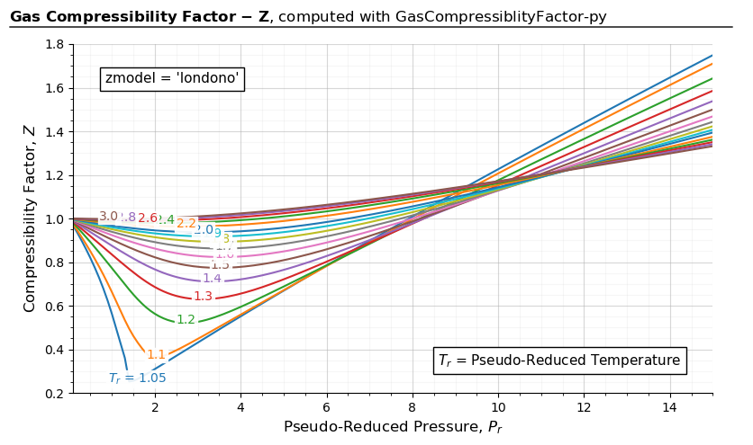
import gascompressibility as gc

results, fig, ax = gc.quickstart(zmodel='londono', prmin=0.2, prmax=15, figsize=(8, 5))
ax.set_ylim(0.2, 1.8)
import gascompressibility as gc

results, fig, ax = gc.quickstart(zmodel='hall_yarborough', prmin=0.2, prmax=15, figsize=(8, 5))
ax.set_ylim(0.2, 1.8)
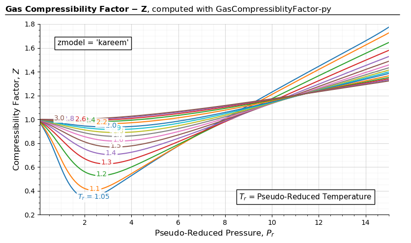
import gascompressibility as gc

results, fig, ax = gc.quickstart(zmodel='kareem', prmin=0.2, prmax=15, figsize=(8, 5))
ax.set_ylim(0.2, 1.8)
For 0.2 < \(P_{r}\) < 30:
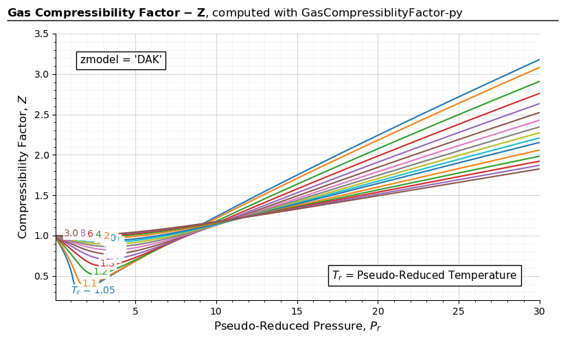
import gascompressibility as gc

results, fig, ax = gc.quickstart(zmodel='DAK', prmin=0.2, prmax=30, figsize=(8, 5))
ax.set_ylim(0.2, 3.5)
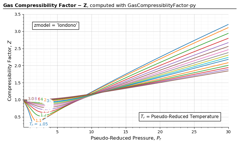
import gascompressibility as gc

results, fig, ax = gc.quickstart(zmodel='londono', prmin=0.2, prmax=30, figsize=(8, 5))
ax.set_ylim(0.2, 3.5)
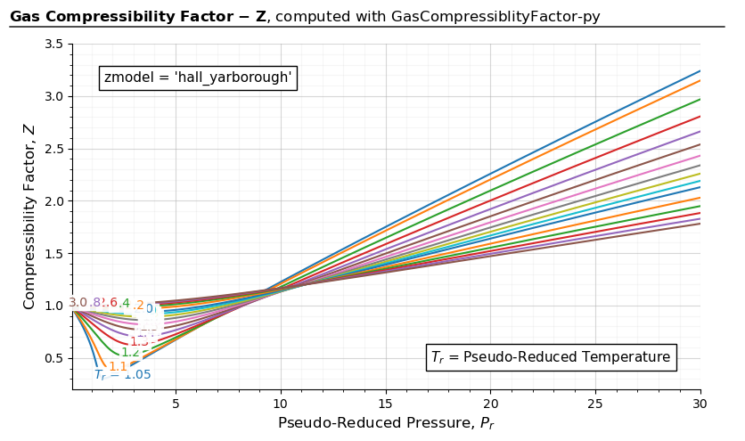
import gascompressibility as gc

results, fig, ax = gc.quickstart(zmodel='hall_yarborough', prmin=0.2, prmax=30, figsize=(8, 5), guess=2)
ax.set_ylim(0.2, 3.5)
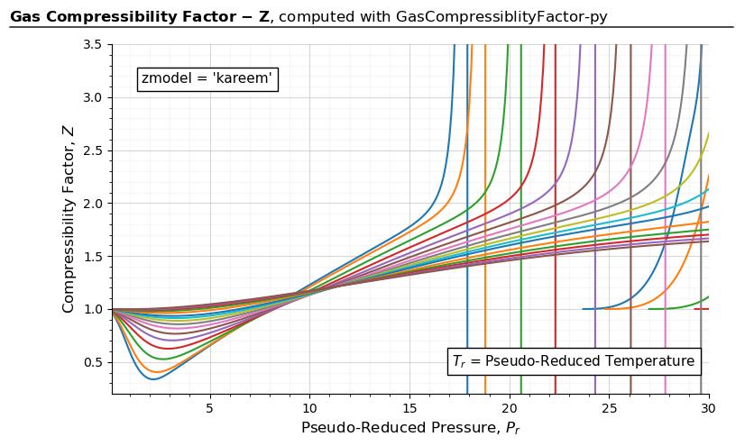
import gascompressibility as gc

results, fig, ax = gc.quickstart(zmodel=kareem, prmin=0.2, prmax=30, figsize=(8, 5), disable_tr_annotation=True)
ax.set_ylim(0.2, 3.5)
2.6. Caveats#
Z-factor correlation models that rely on iterative convergence share issues of their optimization methods - the result depends on the quality of the initial guess. Most times this issues is restricted only to the speed, but sometimes it has direct impact on the final values computed.
Consider the following example when Pr=2.8 and Tr=1.1:
>>> import gascompressibility as gc
>>>
>>> gc.calc_z(Pr=2.8, Tr=1.1, zmodel='hall_yarborough', smart_guess=False, guess=0.9)
0.6001600275325583
>>>
>>> gc.calc_z(Pr=2.8, Tr=1.1, zmodel='hall_yarborough', smart_guess=False, guess=0.1)
0.44138121739974145
When smart_guess is turned off, the computed z value for the hall_yarborough model returns different results despite the same Pr and Tr input
values. The only differences are the guess values. Comparing with the other z-models, we know that the true solution sits around ~0.44.
>>> gc.calc_z(Pr=2.8, Tr=1.1, zmodel='DAK', smart_guess=False, guess=0.9)
0.44245159219674585
>>>
>>> gc.calc_z(Pr=2.8, Tr=1.1, zmodel='kareem')
0.42052851684415665
This discrepancy happens because the iterative z-models implemented in GasCompressibility-py ('DAK' | 'hall_yarborough' | 'londono')
rely on scipy.optimize.newton method to find a root, and as the official scipy documentation states,
“there is no guarantee that a root has been found. Consequently, the result should be verified.”
Fortunately, GasCompressibility-py has a built-in feature that prevents these rare corner cases by setting smart_guess=True
(default). Observe that the 'hall_yarborough' model is able to converge to the ~0.44 z-factor solution when smart guess is activated:
>>> gc.calc_z(Pr=2.8, Tr=1.1, zmodel='hall_yarborough', smart_guess=True)
0.44138121739974157
The below figure demonstrates some corner cases in which scipy fails converge to the right solution when
smart_guess=False.
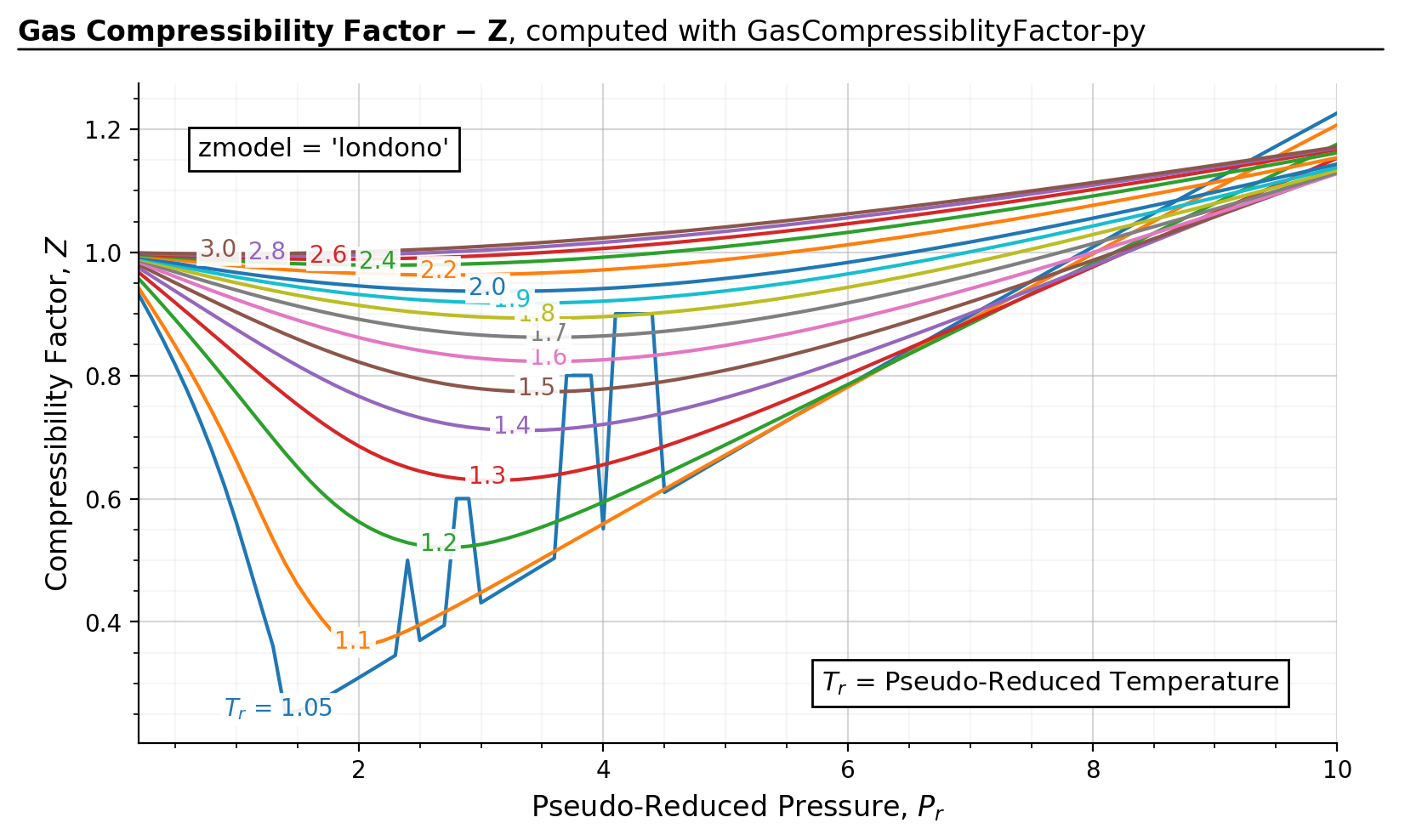
Figure source code
import gascompressibility as gc

results, fig, ax, = gc.quickstart(zmodel='londono', prmin=0.2, prmax=10, smart_guess=False)
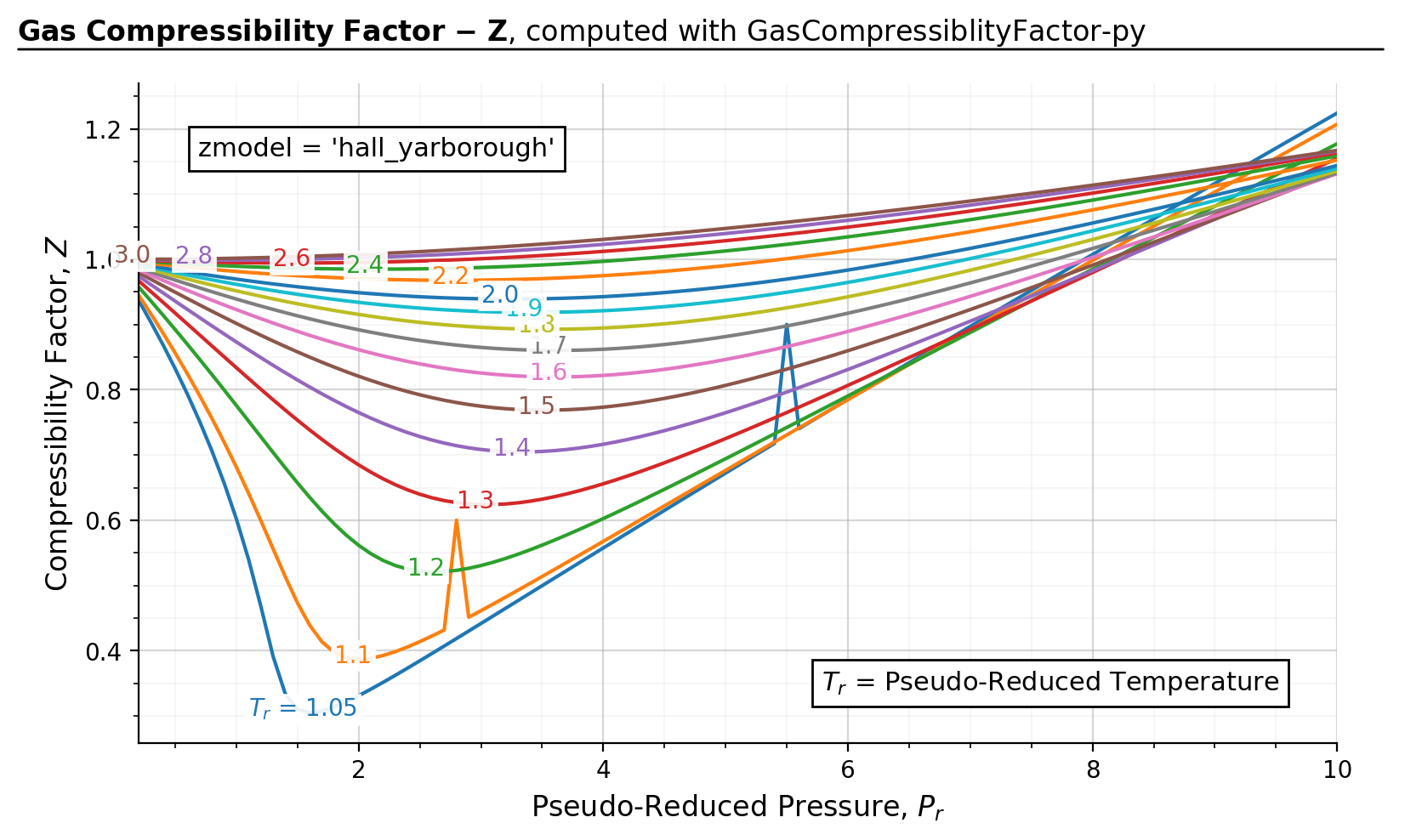
Figure source code
import gascompressibility as gc

results, fig, ax = gc.quickstart(zmodel='hall_yarborough', prmin=0.2, prmax=10, smart_guess=False)
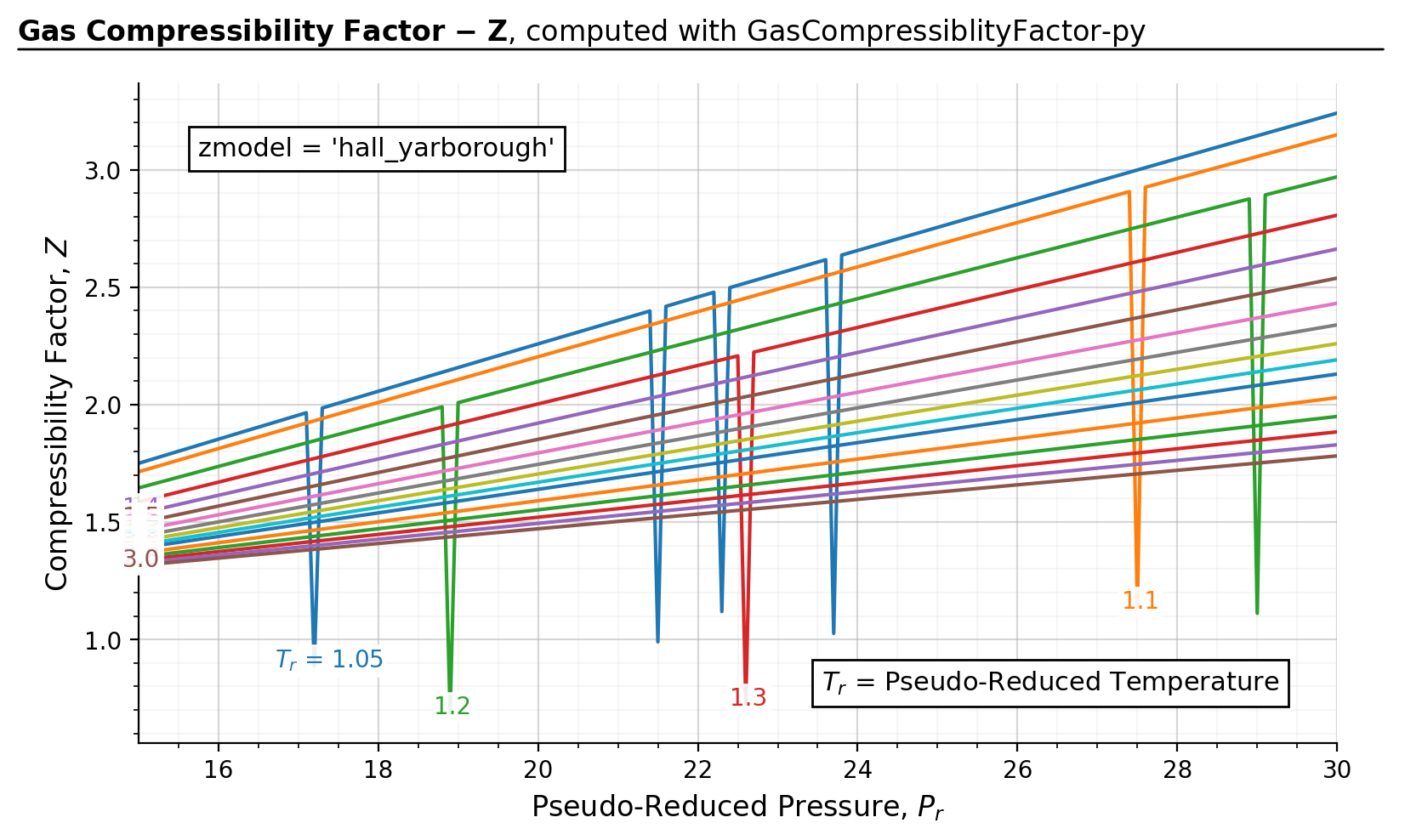
Figure source code
import gascompressibility as gc

results, fig, ax = gc.quickstart(zmodel='hall_yarborough', prmin=15, prmax=30, smart_guess=False)
About smart_guess
smart_guess is a built-in feature activated by default (True) in the
gascompressibility.calc_z function. It provides “smart” initial guess for the z-factor by using
Kareem’s z-model for \(P_r < 15\) (working range of the model). This has two advantages.
Faster because less iterations are needed. Kareem’s model uses an explicit method that doesn’t need iterative convergence.
It’s guaranteed to converge to the correct solution since the guess provided by Kareem’s method should be VERY close to the true solution
For \(P_r > 15\), I found that a guess value of guess=2 (default when Pr > 15) works very well. So far I did not observe any cases in which the function converges to a false solution.
See also
3. What models should I use?#
Short Answer: For z-correlation model, use zmodel='londono'. But if computational cost is a big concern,
use zmodel='kareem' for \(P_r < 15\). For pseudo-critical property model, use pmodel='sutton'. If you have
significant nitrogen fractions, use pmodel='piper'.
3.1. Working Ranges of Z-Models#
The below table summarizes the working \(P_r\) and \(T_r\) ranges of each model, according to it’s own original paper.
Model |
\(T_r\) |
\(P_r\) |
|---|---|---|
DAK |
[1, 3] |
[0.2, 30] |
Hall-Yarborough |
[1.15, 3] |
(0, 20.5] |
Londono |
[1, 3] |
[0.2, 30] |
Kareem |
[1.15, 3] |
[0.2, 15] |
something
However, normally we don’t know the \(P_r\) and \(T_r\) values of a given mixture. The below figure summarizes
the corresponding \(P_r\) and \(T_r\) (computed with Sutton’s method) for each of specific gravity, temperature, and pressure ranges. For
example, assuming \(\gamma_{g}\) = 0.9 (green lines), z-factor correlation can’t be used for extreme conditions like
\(P\) > 19,000 psia, or \(T\) > 800 °F. If Kareem’s method (zmodel='kareem') is used for speed, you can’t
use it for \(P\) > 11,500 psia.
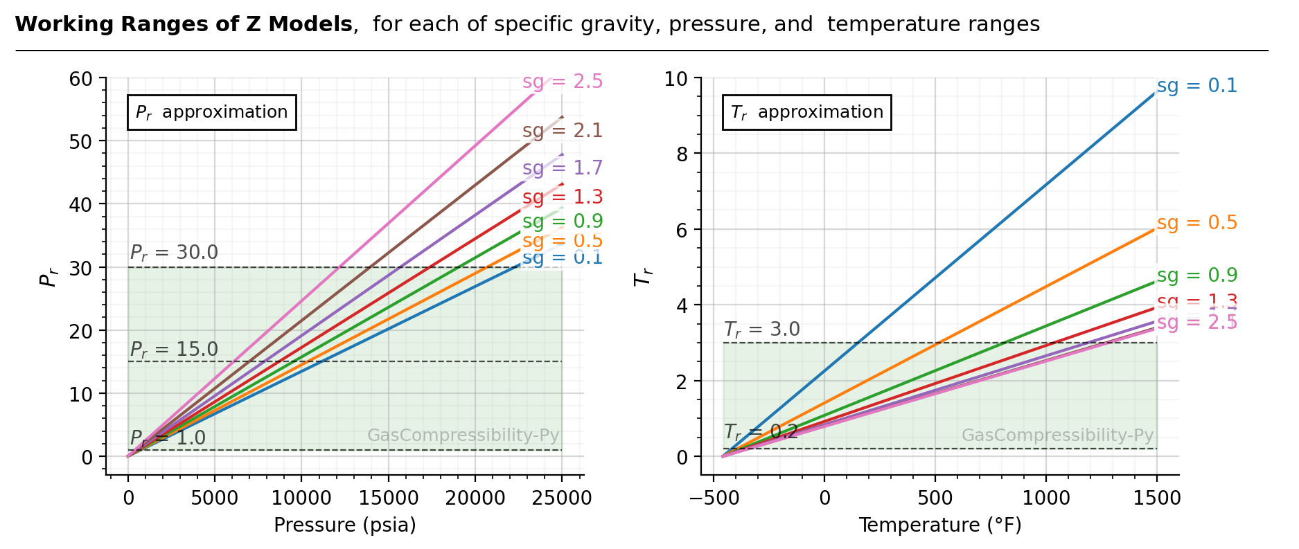
Figure source code
import matplotlib.pyplot as plt
import numpy as np
from gascompressibility.pseudocritical import Sutton

pmin = 0
pmax = 25000
Ps = np.linspace(pmin, pmax, 100)
Ps = np.array([round(P, 1) for P in Ps])

tmin = -459
tmax = 1500
Ts = np.linspace(tmin, tmax, 100)
Ts = np.array([round(T, 1) for T in Ts])

sgs = np.arange(0.1, 2.6, 0.4)
sgs = np.array([round(sg, 1) for sg in sgs])

results = {sg: {
    'Pr': np.array([]),
    'P': np.array([]),
    'Tr': np.array([]),
    'T': np.array([]),
} for sg in sgs}

for sg in sgs:
    for P in Ps:
        Pr = Sutton().calc_Pr(sg=sg, P=P)
        results[sg]['P'] = np.append(results[sg]['P'], [P], axis=0)
        results[sg]['Pr'] = np.append(results[sg]['Pr'], [Pr], axis=0)
    for T in Ts:
        Tr = Sutton().calc_Tr(sg=sg, T=T)
        results[sg]['T'] = np.append(results[sg]['T'], [T], axis=0)
        results[sg]['Tr'] = np.append(results[sg]['Tr'], [Tr], axis=0)

fig, axes = plt.subplots(1, 2, figsize=(9, 4))
for i, ax in enumerate(axes):
    if i == 0:
        for sg in sgs:
            Prs = results[sg]['Pr']
            Ps = results[sg]['P']

            p = ax.plot(Ps, Prs, label=sg)

            t = ax.text(Ps[-10], max(Prs) - 3, 'sg = ' + str(sg), color=p[0].get_color())
            t.set_bbox(dict(facecolor='white', alpha=0.7, edgecolor='white', pad=1))

        ax.text(0.06, 0.9, '$P_{r}$  approximation', fontsize=9, transform=ax.transAxes,
            bbox=dict(facecolor='white'))
        ax.set_ylabel('$P_r$', fontsize=11)
        ax.set_xlabel('Pressure (psia)')
        ymax = 60
        ax.hlines(y=30, xmin=pmin, xmax=pmax, color='k', linestyle='--', linewidth=0.8, alpha=0.7)
        ax.text(100, 31.3, '$P_r$ = 30.0', alpha=0.7)
        ax.hlines(y=15, xmin=pmin, xmax=pmax, color='k', linestyle='--', linewidth=0.8, alpha=0.7)
        ax.text(100, 16, '$P_r$ = 15.0', alpha=0.7)
        ax.hlines(y=1, xmin=pmin, xmax=pmax, color='k', linestyle='--', linewidth=0.8, alpha=0.7)
        ax.text(100, 2, '$P_r$ = 1.0', alpha=0.7)
        ax.fill_between(x=Ps, y1=1, y2=30, color='green', interpolate=True, alpha=0.1, zorder=-99)

    else:
        for sg in sgs:
            Trs = results[sg]['Tr']
            Ts = results[sg]['T']

            p = ax.plot(Ts, Trs, label=sg)

            t = ax.text(Ts[-1], max(Trs), 'sg = ' + str(sg), color=p[0].get_color())
            t.set_bbox(dict(facecolor='white', alpha=0.7, edgecolor='white', pad=1))

        ax.text(0.06, 0.9, '$T_{r}$  approximation', fontsize=9, transform=ax.transAxes,
            bbox=dict(facecolor='white'))
        ax.set_ylabel('$T_r$', fontsize=11)
        ax.set_xlabel('Temperature (°F)')
        ymax = 10
        ax.hlines(y=3, xmin=tmin, xmax=tmax, color='k', linestyle='--', linewidth=0.8, alpha=0.7)
        ax.text(tmin, 3.2, '$T_r$ = 3.0', alpha=0.7)
        ax.hlines(y=0.2, xmin=tmin, xmax=tmax, color='k', linestyle='--', linewidth=0.8, alpha=0.7)
        ax.text(tmin, 0.5, '$T_r$ = 0.2', alpha=0.7)
        ax.fill_between(x=Ts, y1=0.2, y2=3, color='green', interpolate=True, alpha=0.1, zorder=-99)


    ymin = 0 - 0.05 * ymax
    ax.set_ylim(ymin, ymax)

    ax.minorticks_on()
    ax.grid(alpha=0.5)
    ax.grid(visible=True, which='minor', alpha=0.1)
    ax.spines.top.set_visible(False)
    ax.spines.right.set_visible(False)


    def setbold(txt):
        return ' '.join([r"$\bf{" + item + "}$" for item in txt.split(' ')])

    bold_txt = setbold('Working Ranges of Z Models')
    plain_txt = ',  for each of specific gravity, pressure, and  temperature ranges'

    fig.suptitle(bold_txt + plain_txt,
                 verticalalignment='top', x=0, horizontalalignment='left', fontsize=11)
    yloc = 0.9
    ax.annotate('', xy=(0.01, yloc), xycoords='figure fraction', xytext=(1.02, yloc),
                arrowprops=dict(arrowstyle="-", color='k', lw=0.7))
    ax.text(0.95, 0.1, 'GasCompressibility-Py', fontsize=9, ha='right', va='center',
            transform=ax.transAxes, color='grey', alpha=0.5)

fig.tight_layout()
3.2. Compatibilities#
GasCompressibility-py currently supports two pseudo-critical models ('sutton' | 'piper') and four z-factor
correlation models ('DAK' | 'hall_yarborough' | 'londono' | 'kareem'). Which combination of
pseudo-critical model should you use with which z-factor correlation model? The below table presented in Elsharkawy and
Elsharkawy (2020) [12] may shed light on determining which combination should be used:
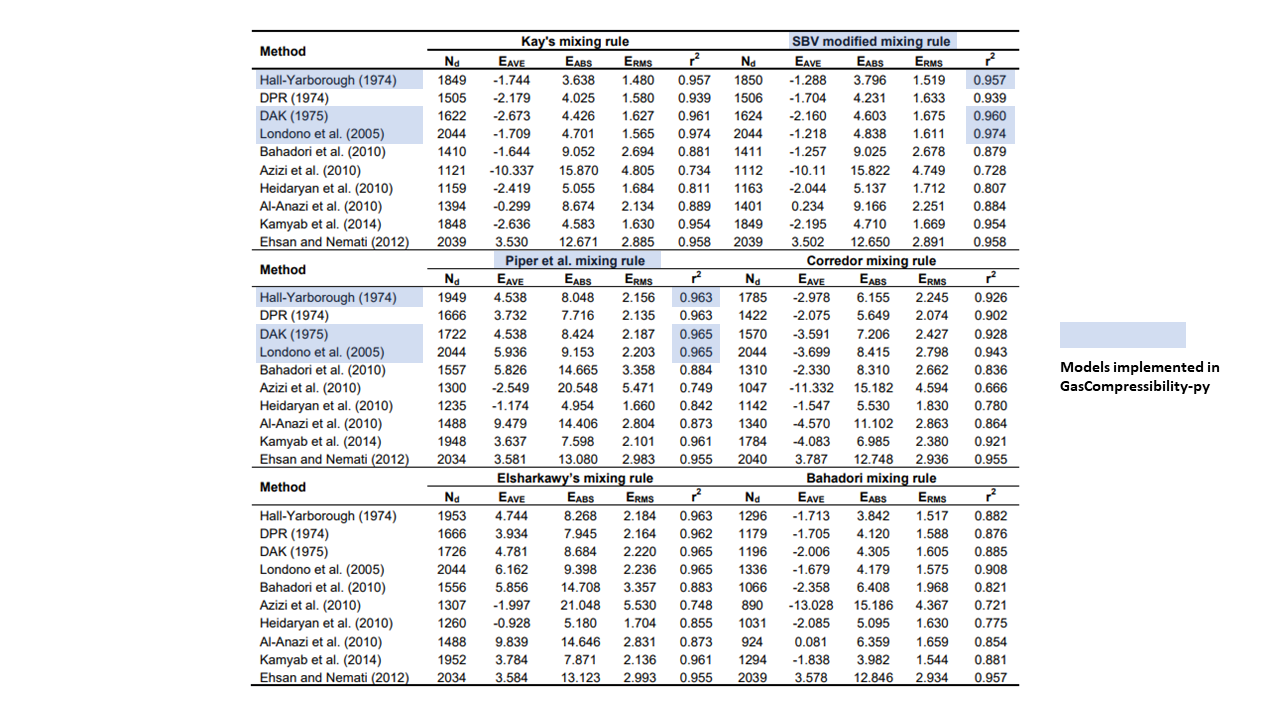
The table dictates that Sutton’s pseudo-critical property model with Londono’s z-factor correlation model yields the highest coefficient of determination (\(R^2\)) of 0.974. However, so long as the models implemented in this package are concerned, you can use any combination you want. They all have \(R^2 \geq 0.957\), which is more than good enough for practical usage in real life applications.
Notes
Unfortunately this performance evaluation table does not include any explicit (fast) z-factor correlation models. Therefore, my recommendation is to avoid Kareem’s method unless computation speed is very important, since there’s no 3rd party paper (that I know of) that evaluates Kareem’s method other than himself.
3.3. Brief Of Each Models#
Pseudo-critical models:
Sutton (1985): Makes corrections for acid fractions: \(H_2S\) and \(CO_2\)
Piper (1993): Improved version of Piper. Additionally supports corrections for \(N_2\) along with \(H_2S\) and \(CO_2\)
Z-factor models:
DAK (1975): The most widely used z-factor model in the oil and gas industry for the past 40 years. You can’t go wrong with this model
Hall-Yarborough (1973): Not recommended.
Londono (2005): Improved version of DAK. Math is exactly the same, but regression coefficients are fitted with 4x more data points.
Kareem (2016): Fast, but have shorter working ranges (\(P_r < 15\))